Comparing One and Two means

Lab 6 Set Up

Posit Cloud Set Up

Just as in previous labs, you will need to follow this link to set up Lab 6 in your Posit Cloud workspace:

Link to Set up Lab 6 Hypothesis Tests Part 1 Means

Important

After you have set up Lab 6 using the link above, do not use that link again as it may reset your work. The set up link loads fresh copies of the required files and they could replace the files you have worked on.

Instead use this link to go to Posit Cloud to continue to work on lab 6: Link

RStudio Desktop Setup

Link to download the Lab 6 materials to RStudio Desktop

Note that you will do all your work for this Rehearse 1 in the Lab-6-Rehearse 1 worksheet, so click on that to open it in the Editor window in your RStudio/Posit Cloud Lab 6 Hypothesis Tests 1 workspace.

Comparing One Mean to a Point Value

By “one sample - one mean” our intent is to test whether the mean of a numerical variable in a sample is different from a standard or stated value. From this we want to make an inference about the target population’s mean.

Attribution: The one-sample one mean example is based upon the explanation of the Infer Package update: Infer

Load Packages

First load the necessary packages:

CC1

library(tidyverse)
library(infer)

Inspect the Data

In this example, we are using the gss data set which is included in the Infer package. It is derived from the General Social Survey and is a sample of 500 responses to questions on the larger survey. You can find information about the GSS here.

Because the gss data set is included in Infer package which we have already loaded into the session library, we do not need to load it separately. But we need to create a data object from the gss for consistency with our process.

CC2

gss <- gss
# Use the glimpse () function to display the data object.
glimpse(gss)

## Rows: 500
## Columns: 11
## $ year    <dbl> 2014, 1994, 1998, 1996, 1994, 1996, 1990, 2016, 2000, 1998, 20…
## $ age     <dbl> 36, 34, 24, 42, 31, 32, 48, 36, 30, 33, 21, 30, 38, 49, 25, 56…
## $ sex     <fct> male, female, male, male, male, female, female, female, female…
## $ college <fct> degree, no degree, degree, no degree, degree, no degree, no de…
## $ partyid <fct> ind, rep, ind, ind, rep, rep, dem, ind, rep, dem, dem, ind, de…
## $ hompop  <dbl> 3, 4, 1, 4, 2, 4, 2, 1, 5, 2, 4, 3, 4, 4, 2, 2, 3, 2, 1, 2, 5,…
## $ hours   <dbl> 50, 31, 40, 40, 40, 53, 32, 20, 40, 40, 23, 52, 38, 72, 48, 40…
## $ income  <ord> $25000 or more, $20000 - 24999, $25000 or more, $25000 or more…
## $ class   <fct> middle class, working class, working class, working class, mid…
## $ finrela <fct> below average, below average, below average, above average, ab…
## $ weight  <dbl> 0.8960034, 1.0825000, 0.5501000, 1.0864000, 1.0825000, 1.08640…

In the glimpse, we can see that the gss data object has 500 rows or observations of the variables. The variables are stored in the columns and we can see we have 11 variables.

See Glimpse for an explanation of the terms used.

Our variable of interest is the ‘hours’ variable which is quantitative. It represents the number of hours worked each week by the individuals who participated in the GSS survey.

Exploratory data analysis

Visualize the data

We will show the distribution of the data using a histogram. We have added code to calculate the mean hours worked per week and to show it on the graph with a dashed line.

CC3

ggplot(gss, aes(x = hours)) +
  geom_histogram(binwidth = 5, fill = "#69b3a2", color = "#e9ecef") +
  geom_vline(aes(xintercept = mean(hours)), 
      color = "black", linetype = "dashed", size = 1) +
  annotate("text", x = mean(gss$hours), y = 130, 
      label = paste("Mean:", round(mean(gss$hours), 3)),
           size = 5, hjust = -.25) +
  scale_x_continuous(breaks = seq(0, max(gss$hours), by = 5),
  labels = seq(0, max(gss$hours), by = 5)) + 
  theme_light()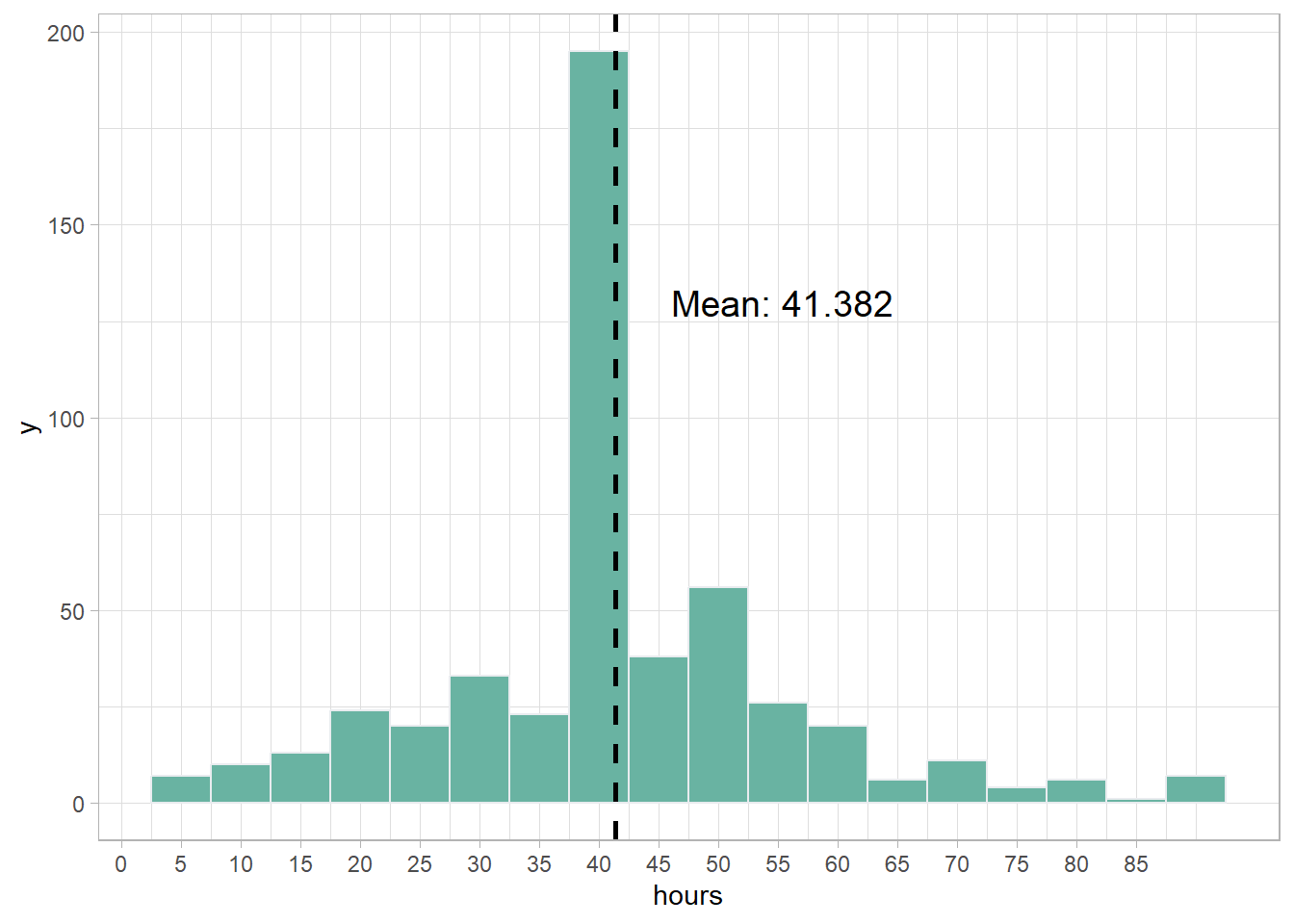

The distribution of hours in the sample has a peak near 40 hours. However, there are long tails in both directions showing a large variation in the hours worked per week by the people responding to the survey. The range is from less than 5 hours per week to more than 85 hours per week.

The mean hours worked per week in our sample is 41.382 hours per week. This seems to indicate that Americans, on average, work more than 40 hours per week.

But this is just a sample and not the entire population of American workers. So, we must take into account the variation in hours worked per week in the sample.

We do this by performing a hypothesis test on the sample data.

State the research question

Does the GSS survey provide sufficient evidence to conclude that the mean number of hours worked each week by Americans is greater than the traditional 40 hour week?

In the Null Hypothesis Significance Test (NHST), the claim, or what the researchers believe or want to prove, is stated in the Alternative Hypothesis.

The Null Hypothesis always is the exact opposite of the Alternative. Because they are exact opposites, only one can be true. If the Null is true, the Alternative must be false. If the Null is false, the Alternative must be true.

Important Concept: The goal of hypothesis testing is to gather evidence against the Null in favor of the Alternative hypothesis.

State the Null and Alternative hypotheses

Null Hypothesis, Ho: The mean hours per week worked by Americans is less than or equal to 40.

Alternative Hypothesis, Ha: The mean hours per week worked by Americans is greater than 40.

We have stated the Null and Alternative in a “directional” format because we are interested in knowing if the mean number of hours worked per week by Americans is greater than 40. If you think of a number line, than we are interested in “proving” that mean hours worked falls to the right of 40 as it does in the histogram.

If on the other hand, we were interested in showing that Americans work fewer hours than 40 per week, the hyptotheses would be stated this way:

Null Hypothesis, Ho: The mean hours per week worked by Americans is greater than or equal to 40.
Alternative Hypothesis, Ha: The mean hours per week worked by Americans is less than 40.

This would be a “less than” or “left-tail” test.

And if we just believed that Americans do not work 40 hours per week, we would state the hypotheses this way:

Null Hypothesis, Ho: The mean hours per week worked by Americans is equal to 40.
Alternative Hypothesis, Ha: The mean hours per week worked by Americans is not equal to 40.

This would be a non-directional or “both tails” test.

Important Concept: The Null Hypothesis is always a form of “no difference” or “equality.”

Important Concept: The direction of the test is determined by the Alternative Hypothesis.

Because in this example the Alternative Hypothesis contains the phrase “greater than”, this is a “right-tail” test. If we wrote the hypotheses using math symbols, the Alternative would have the > symbol. You can think of this as the > pointing to the right.

In this example we will perform the directional, right-tail test.

State the Significance Level

It’s important to set the significance level “alpha” before starting the testing using the data.

Let’s set the significance level at 5% ( i.e., 0.05) here because nothing too serious will happen if we are wrong.

Test the hypothesis - Downey Method

Here’s how we use the Downey method with infer package to conduct this hypothesis test:

Step 1: Calculate the observed statistic

Calculate the observed statistic and store the results in the data object called delta_obs. This is the mean of the sample data.

Although this observed statistic is not really a difference (a delta), we continue to use the delta_obs data object name for consistency with our Downey/Infer process.

Because we are just interested in a single mean, we only need to specify our response variable hours. The test statistic we are using is the mean.

CC4

# When reusing this code chunk in a Remix assignment: 
 # The `delta_obs` data object name should not be changed.
 # Change `gss` to your data set name.
 # change `hours` to your numerical variable.

delta_obs <- gss %>%
  specify(response = hours) %>%
  calculate(stat = "mean") 

delta_obs

## Response: hours (numeric)
## # A tibble: 1 × 1
##    stat
##   <dbl>
## 1  41.4

Step 2: Generate the Null Distribution

Generate the null distribution of the mean hours. We use the null_dist data object to hold this data.

We will hypothesize a Null single “point” mean value of 40. We use 40 as the Null value because the Null is correct if the mean is 40 or less.

CC5

# When reusing this code in a Remix assignment:
 # The `null_dist` data object name should not be changed.
 # Change `gss` to your data set name.
 # change `hours` to your numerical variable.
 # Change the assumed mean value of 40 to your Null value.
 # Do not change anything else.

# set a seed value for reproducible results.
set.seed(123)

# Mu stands for the assumed mean
null_dist <- gss %>%
  specify(response = hours) %>%
  hypothesize(null = "point", mu = 40) %>%
  generate(reps = 1000) %>% 
  calculate(stat = "mean")

# Print first 5 rows
null_dist %>% 
  slice(1:5)

## Response: hours (numeric)
## Null Hypothesis: point
## # A tibble: 5 × 2
##   replicate  stat
##       <int> <dbl>
## 1         1  39.1
## 2         2  39.5
## 3         3  39.6
## 4         4  39.7
## 5         5  43.0

Step 3: Visualize the Null and the Observed Statistic

Here we will plot the distribution of means in null-dist and and the observed test statistic delta_obs.

CC6

# When reusing this code chunk in a Remix assignment, edit only
  # the axis labels, 
  # the title, 
  # and the subtitle. 
  # direction should be for the Alternative hypothesis which is "greater" than in this example.

visualize(null_dist) +
  shade_p_value(obs_stat = delta_obs, direction = "greater")+
  labs(x = "Mean Hours Worked", y = "Count",
       title = "Null distribution of mean hours worked",
       subtitle = "Actual mean hours worked observed (delta_obs) in the data is marked in red"
       ) +
theme_light()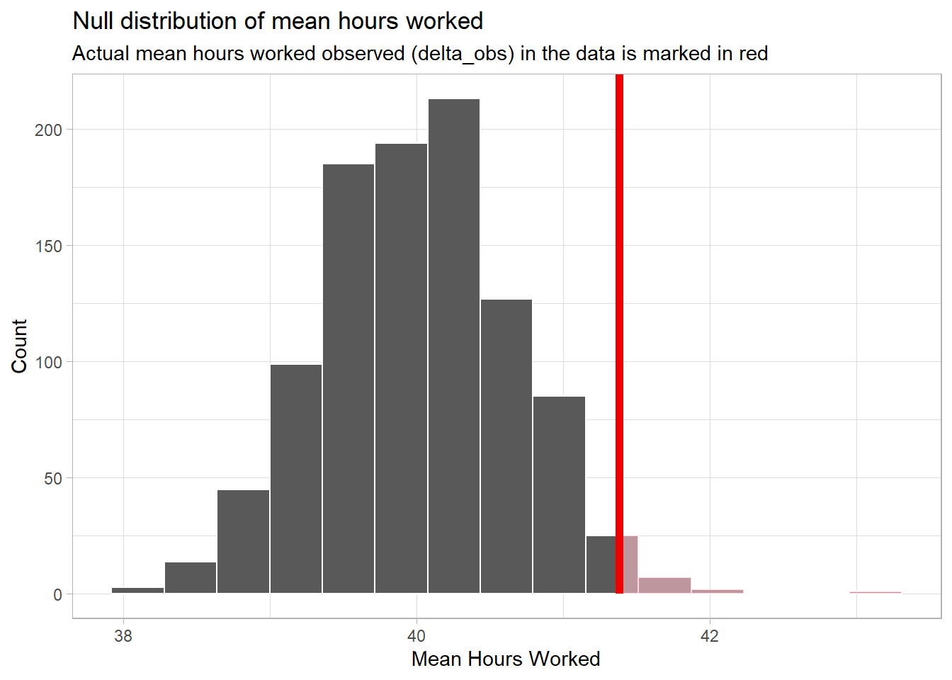

Because this is a directional, right-tail test, we include the “direction = greater” in the above code. If it were a non-directional, two-tail test, we would use “direction = both.” If it were a left-tail test, we would use “direction = less”.

The “Count” on the y-axis is the number of means in the null_dist with a specific value of hours worked. You can see that we do have a “bell-shaped” distribution with the center clustered around 40 and with few observations below 38 or above 42 hours.

Notice that the “pink area under the curve” is only on the right side beyond the red line.

Question: Is the observed sample mean (delta_obs) unlikely to happen often in the Null world? Support your answer by explaining why you think this?

Answer here:

Step 4: Calculate the p-value

Calculate the p-value - the “area” under the curve (the distribution of means in the Null world (in null_dist) beyond the observed sample mean delta_obs. Again, notice this is the pink area on the right side of the red line in the graph.

CC7

# When reusing this code chunk in a Remix assignment, change only the direction to correspond with the alternative hypothesis. Here it is > 40, so "right" or "greater".

p_value <- null_dist %>%
  get_p_value(obs_stat = delta_obs, direction = "greater")

p_value

## # A tibble: 1 × 1
##   p_value
##     <dbl>
## 1   0.015

Similar to Step 3, we set “direction =” to match the Alternative hypothesis.

Step 5: Decide if delta_obs is statistically significant

CC8

# When reusing this code chunk in a Remix assignment:
 # Replace the value for alpha with your significance level

alpha <- 0.05 

if(p_value < alpha){ 
  print("Reject the Null Hypothesis")
} else { 
    print("Fail to reject the Null Hypothesis") 
}

## [1] "Reject the Null Hypothesis"

Although we illustrate making the decision on the p-value using code, you can do this with just logical thinking if you prefer. But do remember that a p-value greater than or equal to the significance level means “Fail to Reject the Null.”

Results and Conclusions

Because we set the significance level alpha to 0.05, the p-value of 0.015 is less than alpha. Thus, the Null hypothesis (mean hours worked <= 40) must be rejected and we can conclude:

The mean number of hours worked each week by Americans is greater than 40.

Calculate confidence interval

The following code chunk creates a 95th percentile confidence interval around the mean hours worked by Americans using the bootstrap method.

CC9

# When reusing this code chunk in a Remix assignment:
 # Change `gss` to your data set.
 # Change `hours` to your numerical variable.
 # Do not change anything else.

# Set seed to make the results reproducible.
set.seed(123)

boot_dist <- gss %>%
   specify(response = hours) %>%
   generate(reps = 1000, type = "bootstrap") %>%
   calculate(stat = "mean")
 
#calculate the 95% confidence interval
ci <- get_ci(boot_dist)

# display the CI
ci

## # A tibble: 1 × 2
##   lower_ci upper_ci
##      <dbl>    <dbl>
## 1     40.1     42.6

Question: State what the confidence interval tells us about the likely mean hours worked per week? Does it support the Null Hypothesis of the mean being less than or equal to 40?

Your Answer here:

Traditional hypothesis test

CC10

# When reusing this code chunk in a Remix assignment:
 # Change hours to your numerical variable..
 # Change gss to your data set
 # Change the Null mean mu of 40 to your value.
 # Change the alternative to less for an Ha using <, or delete that section
 
t.test(gss$hours, mu = 40, alternative = "greater", conf.level = 0.95)

## 
##  One Sample t-test
## 
## data:  gss$hours
## t = 2.0852, df = 499, p-value = 0.01878
## alternative hypothesis: true mean is greater than 40
## 95 percent confidence interval:
##  40.28981      Inf
## sample estimates:
## mean of x 
##    41.382

Again, we include “greater” in the code.

The results of the traditional test are similar to the Infer results. The Null of the mean hours worked being <= 40 must be rejected.

Remember there are assumptions required for the t-test that should be checked and verified before the results can be used. We will not do that here. See Assumptions for Traditional Tests

Comparing Two Means

When we need to determine whether there is a significant difference between the means of two groups, there are two types of hypothesis tests we can use: the independent samples test and the paired samples test.

Independent Samples Test: This test is used when you want to compare the means of two independent groups to determine whether there is statistical evidence that the associated population means are significantly different. The two groups are independent, meaning that they do not affect each other. For example, you might use an independent samples test to determine whether there is a difference in exam scores between students who had studied alone versus those who studied in groups.
Paired Samples Test: This test, also known as the dependent samples test, is used when you want to compare the means of the same group or item under two separate scenarios. The two scenarios are dependent, meaning that they are related or paired in some way. For example, you might use a paired samples test to determine whether there is a significant difference in a person’s heart rate before and after consuming caffeine.

In summary, the key difference between these two tests lies in the nature of the samples. Independent samples are separate and unrelated, while paired samples are related in some way. The choice of test depends on the design of your study and the nature of your data.

Independent Samples Test

In Module 5, Rehearse 2, Question 1, we used the Downey-Infer process to test for the difference in the means of two independent samples. The research question was Is there a significant difference in the mean female and male college freshman GPAs?

Note we will not repeat that information here.

Paired Samples Test

Load Packages

First load the necessary packages:

CC11

library(tidyverse)
library(infer)

Inspect the Data

Load the data.

For this example, we will be using data from research on 10 mice who were given a treatment intended to cause them to gain weight. The data file weights.xlsx is in the /data folder.

CC12

# The `readxl` package is needed to load Excel worksheets.
library(readxl)

weights <- read_excel("./data/weights.xlsx")

glimpse(weights)

## Rows: 20
## Columns: 4
## $ ...1   <dbl> 1, 2, 3, 4, 5, 6, 7, 8, 9, 10, 11, 12, 13, 14, 15, 16, 17, 18, …
## $ group  <chr> "before", "before", "before", "before", "before", "before", "be…
## $ weight <dbl> 200.1, 190.9, 192.7, 213.0, 241.4, 196.9, 172.2, 185.5, 205.2, …
## $ diff   <dbl> 12.8, 22.3, -27.6, 0.0, 12.6, 51.0, 69.8, 18.4, 7.1, -21.5, NA,…

We can see in the glimpse that the data set has 20 observations of the mice in the experiment. And it has 3 variables:

group is a categorical variable with two levels: before and after.
weight is the weight (in grams) of the mice.
diff is the difference between the mice weights (after - before). Note there are just 10 observations of the diff variable.

This data set has been “wrangled” to include the “diff” variable which is needed for use of the Downey-Infer approach to paired samples problems.

State the Research Question

Is there a difference in the “before” and “after” treatment weights of the mice?

Exploratory data analysis

Visualize the data

We will use a box plot to help us visualize the data. We will use the group variable on the x-axis and the weight variable on the y-axis.

CC13

ggplot(weights, aes(x = group, y = weight, fill = group)) + 
  geom_boxplot(alpha = 0.7) +
  labs(title = "Weights before and after treatment",
       x = "Group", y = "Weight(gms)") +
  scale_fill_manual(values = alpha(c("#66c2a5", "red"), 0.5)) +
  stat_summary(
    fun = mean, 
    geom = "point", 
    shape = 18, 
    size = 4, 
    color = "yellow", 
    position = position_dodge(width = 0.75),
    show.legend = FALSE
  ) +  
  theme_light()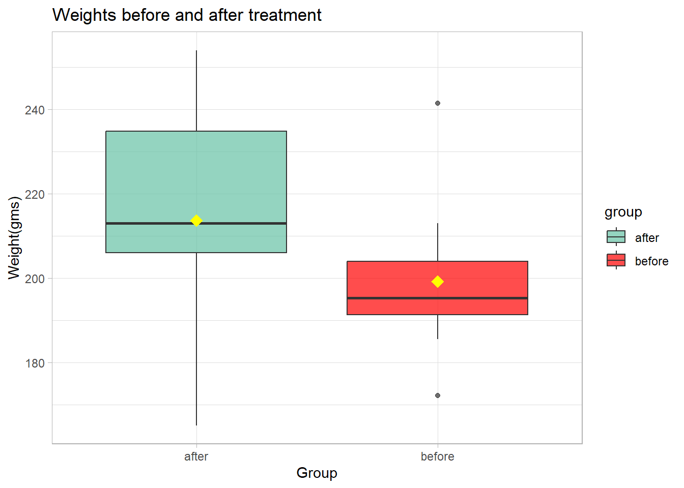

Note the standard boxplot displays the medians which are the black lines near the “middle” of the two boxes. We can see that there is some difference in the median weight for the two groups. The median weight for after appears to be greater than that for before. Our code adds yellow diamonds indicating the means of the two groups.

A boxplot can tell us something about the distribution of the data points but a density plot can often tell more.

CC14

# Calculate means for each group
mean_data <- aggregate(weight ~ group, data = weights, FUN = mean)

ggplot(weights, aes(x = weight, color = group, fill = group)) +
  geom_density(alpha = 0.5) +
  labs(title = "Weights before and after treatment",
       x = "Weight (gms)", y = "Density") +
 geom_vline(data = mean_data, aes(xintercept = weight, color = group), linetype = "dashed", size = 1) +
  annotate("text", x = mean_data$weight, y = 0, label = round(mean_data$weight, 2),
           vjust = -0.5, hjust = 0.5, color = "black", size = 4) +
  theme_minimal()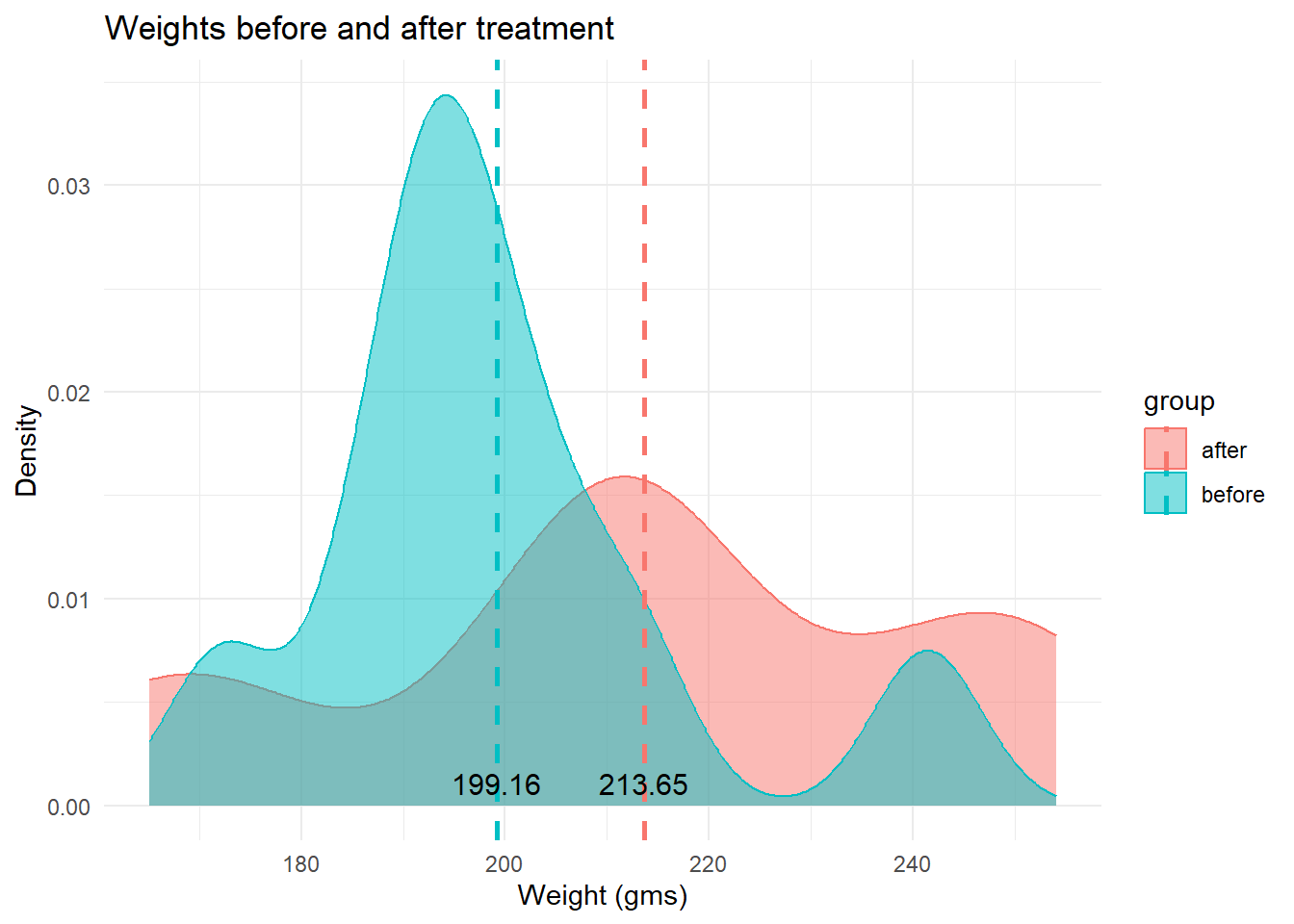

The density plot of the two distributions indicates that the before weights are clustered around a large peak of about 195 grams, with a second, lower peak about 240 grams. The after group has a much lower peak and is more evenly distributed. That said, the two groups overlap each other substantially. The mean weights of the two groups are indicated by dashed lines.

Both graphs do suggest that the mean weight of the after group is greater than that of the before group. The mean of the before group is 199.16 grams and that of the after group is 213.65 grams. But is that difference enough to be statistically significant, given the overlap in the two distributions?

State the Null and Alternative hypotheses

Null Hypothesis Ho: There is no difference in the before treatment and after treatment weights.

Alternative Hypothesis Ha: There is a difference between the before treatment and after treatment weights.

Question: What is the direction of this hypothesis test?

Your answer here:

State the Significance Level

It’s important to set the significance level “alpha” before starting the testing using the data.

Let’s set the significance level at 5% ( i.e., 0.05) here because nothing too serious will happen if we are wrong.

Testing the hypothesis

Step 1: Calculate the observed statistic

Calculate the observed statistic and store the results in a new data object called delta.

Important!

The Infer package functions for conducting a paired samples test require the use of a pre-computed variable representing the calculated differences between the “before” and “after” conditions. In our course data sets, this variable is named ‘diff’. But if you use a dataset that does not have a “diff” variable, you will need to pre-compute it and add that column of values.

CC15

# When reusing this code chunk in a Remix assignment: 
 # The `delta_obs` data object name should not be changed.
 # Change `weights` to your data set name.
 # Change `diff` to your difference variable name
 # No other changes are needed.

delta_obs<- weights %>% 
  specify(response = diff) %>% 
  calculate(stat = "mean")

# Display the observed difference
delta_obs

## Response: diff (numeric)
## # A tibble: 1 × 1
##    stat
##   <dbl>
## 1  14.5

The after group has a mean weight 14.5 grams more than the before group.

Step 2: Generate the Null Distribution

Generate the null distribution of the difference in weights.

CC16

# When reusing this code in a Remix assignment:
 # The `null_dist` data object name should not be changed.
 # Change `weights` to your data set name.
 # Change `diff` to your response variable.
 # No other changes are needed.

set.seed(123)
null_dist <- weights %>% 
  specify(response = diff) %>% 
  hypothesize(null = "paired independence") %>% 
  generate(reps = 1000, type = "permute") %>% 
  calculate(stat = "mean") 

null_dist %>% 
  slice(1:5)

## Response: diff (numeric)
## Null Hypothesis: paired independence
## # A tibble: 5 × 2
##   replicate    stat
##       <int>   <dbl>
## 1         1 -11.6  
## 2         2  11.6  
## 3         3 -17.4  
## 4         4  -0.970
## 5         5  18.8

Note we use the hypothesize function to set our null hypothesis to be “paired independence”. If the two variables group and weight are independent of each other, we should see no difference in the mean weights of the mice before and after the treatment - the diff. We use the calculate function to find the mean of each of the “reps” in the null_dist data object.

Step 3: Visualize the Null and the Observed Statistic

Because this is a non-directional test, we set the “direction =” in the code to “both”.

CC17

# When reusing this code chunk in a Remix assignment, edit only
  # the axis labels, 
  # the title, 
  # and the subtitle. 

visualize(null_dist) +
  shade_p_value(obs_stat = delta_obs, direction = "both") +
  labs(x = "Difference in Weight (grams)", y = "Count", 
       title = "Null distribution of Difference in Mouse Weight before and after treatment",
       subtitle = "Actual difference observed in the sample data is marked in red") +
  theme_light()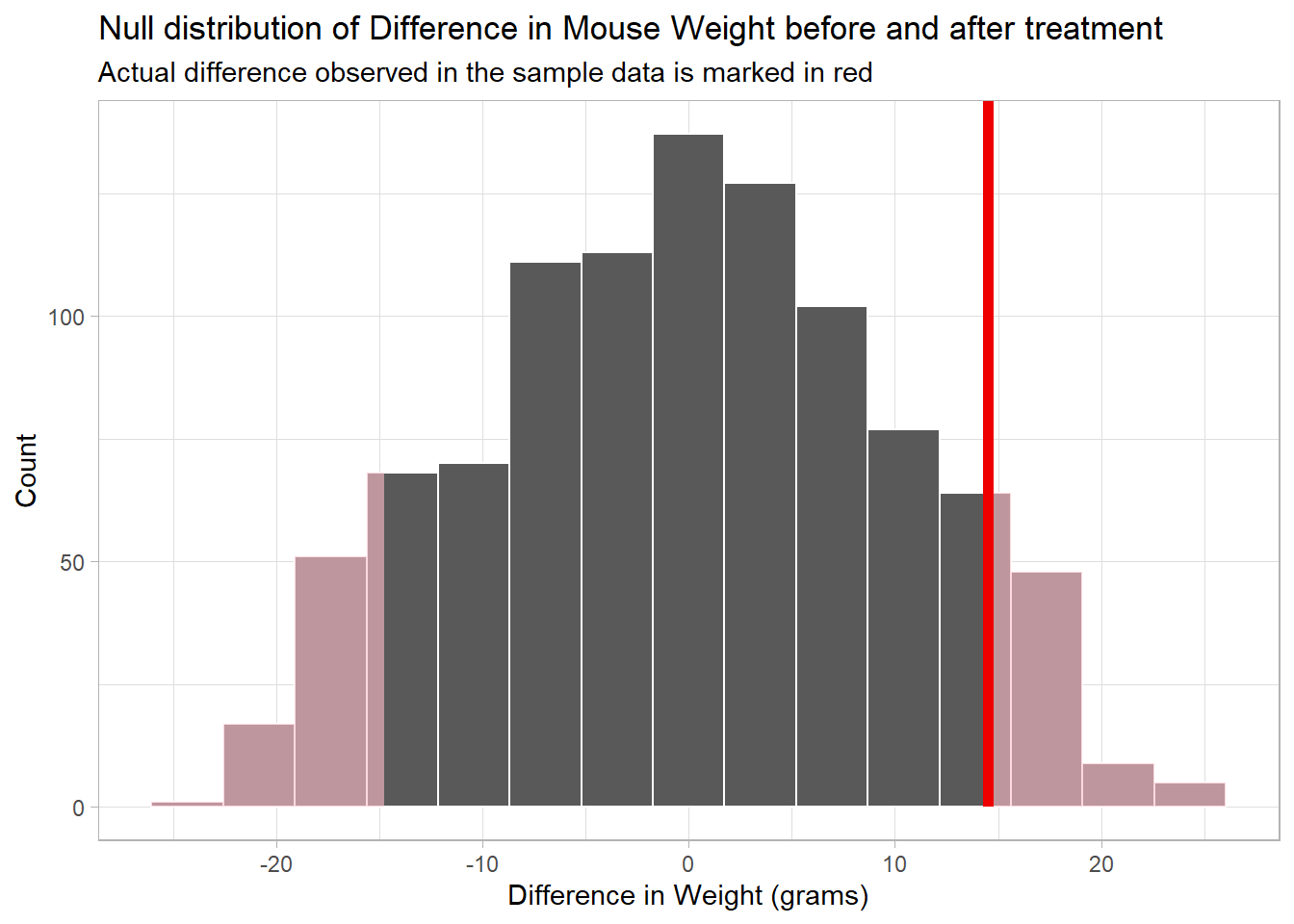

Question: Do you think the observed delta (delta_obs) occurs often in the Null world? Explain your thinking.

Your answer here:

Step 4: Calculate the p-value

Calculate the p-value (“area” under the curve beyond delta_obs) from the Null distribution and the observed statistic delta_obs.

We use the “both” direction because we are interested in a difference either way - a gain or a loss of weight. And that is the “pink” area under the tails in both the negative and positive directions beyond a difference of +14.9 and -14.9 grams.

CC18

#When resuing this code chunk in a Remix assignment, no changes are needed.

p_value <- null_dist %>%
  get_pvalue(obs_stat = delta_obs, direction = "both")

p_value

## # A tibble: 1 × 1
##   p_value
##     <dbl>
## 1   0.164

Step 5: Decide if delta_obs is statistically significant

CC19

# When reusing this code chunk in Remix assignment:

 # Replace the value for alpha with your significance level
 # No other changes are needed.

alpha <- 0.05 

if(p_value < alpha){ 
  print("Reject the Null Hypothesis")
} else { 
    print("Fail to reject the Null Hypothesis") 
}

## [1] "Fail to reject the Null Hypothesis"

Results and Conclusions

Because the p-value of approximately 0.164 is greater than the significance level of 0.05, we cannot reject the Null hypothesis of no difference.

There is no significant difference between the weights of the mice before and after the treatment.

Question: Is the finding of “no difference” surprising to you? Why or why not?

Your answer here:

Question: Do you think the substantial overlap of the distributions of the two groups (shown on the density plot) impacted whether or not the difference was signficant? Explain you thinking.

Your answer here:

Calculate confidence interval

The following code chunk will allow us to calculate a 95% confidence interval for the difference between mean mice weight “after” and “before” the treatment.

CC20

# When reusing this code chunk in a Remix Assignment,
 # Do not change the name `ci`
 # Change `weights` to your data set.
 # Change `diff` to your numerical difference variable.

set.seed(123)

ci <- weights %>% 
  specify(response = diff) %>%
  generate(reps = 1000, type="bootstrap") %>% 
  calculate(stat = "mean") %>% 
  get_confidence_interval(level = 0.95)


#print the CI upper and lower limits
ci

## # A tibble: 1 × 2
##   lower_ci upper_ci
##      <dbl>    <dbl>
## 1    -2.47     32.2

The Null value of 0 is in the confidence interval. This supports the conclusion that there is no significant difference in mice weight before and after the treatment.

Traditional hypothesis test

We can check the results of our Downey-Infer process by running a traditional one sample t-test for the mean difference of 0.

CC21

t.test(weights$diff, mu = 0)

## 
##  One Sample t-test
## 
## data:  weights$diff
## t = 1.5558, df = 9, p-value = 0.1542
## alternative hypothesis: true mean is not equal to 0
## 95 percent confidence interval:
##  -6.578052 35.558052
## sample estimates:
## mean of x 
##     14.49

The traditional one-sample t-test on the diff variable produces similar results.

Because our weights data object also has the original group variable with the “before” and “after” mice weights, we can run a traditional paired samples t-test.

CC22

# When reusing this code chunk in a Remix Assignment:
 # Change weights to your data set.
 # Change weight to your numerical variable.
 # Change group to your categorical variable

t.test(weight ~ group, data = weights, paired = TRUE)

## 
##  Paired t-test
## 
## data:  weight by group
## t = 1.5558, df = 9, p-value = 0.1542
## alternative hypothesis: true mean difference is not equal to 0
## 95 percent confidence interval:
##  -6.578052 35.558052
## sample estimates:
## mean difference 
##           14.49

This traditional paired samples t-test and the traditional single sample t-test for a difference of 0 have essentially identical results. And both are essentially the same results as we got with the Downey-Infer paired samples method.

Question: If the two methods (Downey v traditional) produce almost identical results, why not just use the “simpler” traditional method?

Answer here:

Lab Assignment Submission

Important

When you are ready to create your final lab report, save the Lab-06-Rehearse1-Worksheet.Rmd lab file and then Knit it to PDF or Word to make a reproducible file.

Note that if you have difficulty getting the documents to Knit to either Word or PDF, and you cannot fix it, just save the completed worksheet and submit your .Rmd file for partial credit.

Submit your file in the M6.3 Lab 6 Rehearse(s): Hypothesis Tests Part 1 - Means assignment area.

The Lab 6 Hypothesis Tests Part 2 Grading Rubric will be used.

Congrats! You have finished Rehearse 1 of Lab 6. Now go to Rehearse 2!

Previous: Lab 6 Overview

Next: Lab 6 Rehearse 2

Lab Manual Homepage

This work was created by Dawn Wright and is licensed under a Creative Commons Attribution-ShareAlike 4.0 International License.

v2.1, 12/26/23

Last Compiled 2024-05-26

Lab 6 Rehearse 1

Hypothesis Tests Part 1

Comparing One and Two means

Lab 6 Set Up

Posit Cloud Set Up

RStudio Desktop Setup

Comparing One Mean to a Point Value

Load Packages

Inspect the Data

Exploratory data analysis

Visualize the data

State the research question

State the Null and Alternative hypotheses

State the Significance Level

Test the hypothesis - Downey Method

Step 1: Calculate the observed statistic

Step 2: Generate the Null Distribution

Step 3: Visualize the Null and the Observed Statistic

Step 4: Calculate the p-value

Step 5: Decide if delta_obs is statistically significant

Results and Conclusions

Calculate confidence interval

Traditional hypothesis test

Comparing Two Means

Independent Samples Test

Paired Samples Test

Load Packages

Inspect the Data

State the Research Question

Exploratory data analysis

Visualize the data

State the Null and Alternative hypotheses

State the Significance Level

Testing the hypothesis

Step 1: Calculate the observed statistic

Step 2: Generate the Null Distribution

Step 3: Visualize the Null and the Observed Statistic

Step 4: Calculate the p-value

Step 5: Decide if delta_obs is statistically significant

Results and Conclusions

Calculate confidence interval

Traditional hypothesis test

Lab Assignment Submission