Data Import/Export

Read an R data set

One type of date set often encountered is an R data set. These are datasets that are created in R and saved with an .RData extension. If your dataset, mydata.RData, is stored in your data sub-directory, load the file as an R object:

load("./data/mydata.RData")

Note: the mydata object should be visible in your Environment window. You do not need to assign a dataframe.

Data set from a package

To see a list of all data sets in the package openintro. Note this creates a new tab in the editor window labeled “R data sets”.

library(openintro)
data(package = "openintro")

To create a new data frame, loans, from one of the listed data sets in openintro package, loan50. Note: get data set name from previous step.

loans <- as.data.frame(loan50)

CSV file from URL

Requires the readr library.

Reads csv data file from https URL and assigns to a data frame.

library(readr)
ma_schools <- read_csv("https://docs.google.com/spreadsheets/d/e/2PACX-1vSrWSNyNqRVA950sdYa1QazAT-l0T7dl6pE5Ewvt7LkSm9LXmeVNbCbqEcrbygFmFyK4B6VQQGebuk9/pub?gid=1469057204&single=true&output=csv")

CSV file from local directory

Put path to file inside the quotes. This example is for a data folder in the root folder. If the file is in the root folder, just enter its name without the path, i.e., ./data/

library(readr)
wwbi <- read_csv("./data/WWBIData.csv")

Excel File from local directory

Requires readxl package

Note the file type .xls or .xlsx

library(readxl)
data<- read_excel("./data/DHS_450.xlsx")

Export data frame as csv

#the function needs the name of the data frame, then after the comma, the path and the name for the csv file.

To local root directory.

write.csv(wwbi_small, "wwbi_small.csv")

To the data directory.

write.csv(wwbi_2012, "./data/wwbi_2012.csv")

Export data frame as Excel

This will export to your /data directory. See above for exporting to your root directory. Note may need to install the writexl package first.

library(writexl)
write_xlsx(wwbi_2012, "./data/wwbi_2012.xlsx")

Wrangling Data

Create Data Frame from scratch

Begin by creating three data vectors:

employeename <- c('Sally Green','Paul Smith','Mary Johnston')
salary <- c(54000, 65000, 59500)
hiredate <- as.Date(c('2001-8-21','1999-5-14','2012-10-25'))

Note that the three data vectors are placed in the “Values” section of the Environment rather than in the “Data” section where data tables/frames are placed.

-a character vector named “employeename” which has the names
-a numeric vector named “salary” which has the annual salaries
-a date vector named “hiredate” which is the formal employment date.

Check this blog post out if you want to know more about the types of data used in R: https://statsandr.com/blog/data-types-in-r/

Next we will combine these three data vectors into a data frame/table.

employ.data <- data.frame(employeename, salary, hiredate, stringsAsFactors = FALSE)

Note that R will automatically turn a character vector into a factor unless the “stringsAsFactors = False” is not used.

#Let's look at the table

employ.data

##    employeename salary   hiredate
## 1   Sally Green  54000 2001-08-21
## 2    Paul Smith  65000 1999-05-14
## 3 Mary Johnston  59500 2012-10-25

We can use the str() function to show us the structure of the data frame.

str(employ.data)

## 'data.frame':    3 obs. of  3 variables:
##  $ employeename: chr  "Sally Green" "Paul Smith" "Mary Johnston"
##  $ salary      : num  54000 65000 59500
##  $ hiredate    : Date, format: "2001-08-21" "1999-05-14" ...

Create Table

Using cpr data in openintro package

library(openintro)

cpr

## # A tibble: 90 × 2
##    group   outcome 
##    <fct>   <fct>   
##  1 control survived
##  2 control survived
##  3 control survived
##  4 control survived
##  5 control survived
##  6 control survived
##  7 control survived
##  8 control survived
##  9 control survived
## 10 control survived
## # ℹ 80 more rows

The data set cpr has two factors or variables, group and outcome. Each has two levels. group has control and treatment. outcome has died and survived.

Make table using two variables with two levels each

table(cpr$group, cpr$outcome)

##            
##             died survived
##   control     39       11
##   treatment   26       14

More How-to on making contingency tables

Filter and Select Data

See

Simple and quick explanation: https://blog.exploratory.io/filter-data-with-dplyr-76cf5f1a258e

More details on Filter https://www.r-bloggers.com/2019/04/how-to-filter-in-r-a-detailed-introduction-to-the-dplyr-filter-function/

Graphs

For detailed instructions on creating graphs using the Grammar of Graphics process, see Modern Dive **Five named graphs

This chapter in R for Data Science will show you more easy ways to make your graphs better: Graphics for communication

Also, check out this video which walks you through the typical steps using ggplot2: Visualizing data with ggplot2

Boxplot

library(ggplot2)
library(usdata)

ggplot(county, aes(x = median_edu, y = median_hh_income)) +
  geom_boxplot()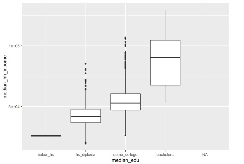

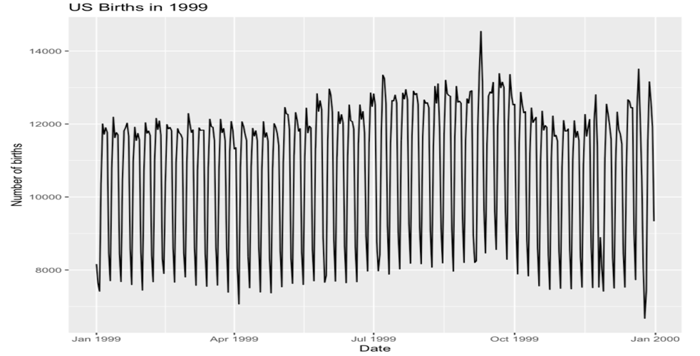
Line graph/Time series

Requires ggplot2 package

ggplot(US_births_1999, aes(x = date, y = births)) +
  geom_line() +
  labs(x = "Date", 
       y = "Number of births", 
       title = "US Births in 1999")

Example

Scatter plot

library(tidyverse)
library(ggplot2)
library(palmerpenguins)
glimpse(penguins)

## Rows: 344
## Columns: 8
## $ species           <fct> Adelie, Adelie, Adelie, Adelie, Adelie, Adelie, Adel…
## $ island            <fct> Torgersen, Torgersen, Torgersen, Torgersen, Torgerse…
## $ bill_length_mm    <dbl> 39.1, 39.5, 40.3, NA, 36.7, 39.3, 38.9, 39.2, 34.1, …
## $ bill_depth_mm     <dbl> 18.7, 17.4, 18.0, NA, 19.3, 20.6, 17.8, 19.6, 18.1, …
## $ flipper_length_mm <int> 181, 186, 195, NA, 193, 190, 181, 195, 193, 190, 186…
## $ body_mass_g       <int> 3750, 3800, 3250, NA, 3450, 3650, 3625, 4675, 3475, …
## $ sex               <fct> male, female, female, NA, female, male, female, male…
## $ year              <int> 2007, 2007, 2007, 2007, 2007, 2007, 2007, 2007, 2007…

ggplot(data = penguins,
  mapping = aes(x = bill_depth_mm, y = bill_length_mm, colour = species)) +
  geom_point() +
  labs(title = "Bill depth and length",
      subtitle = "Dimensions for Adelie, Chinstrap, and Gentoo Penguins", 
      X = "Bill depth (mm)", y = "Bill length (mm)", 
      colour = "Species")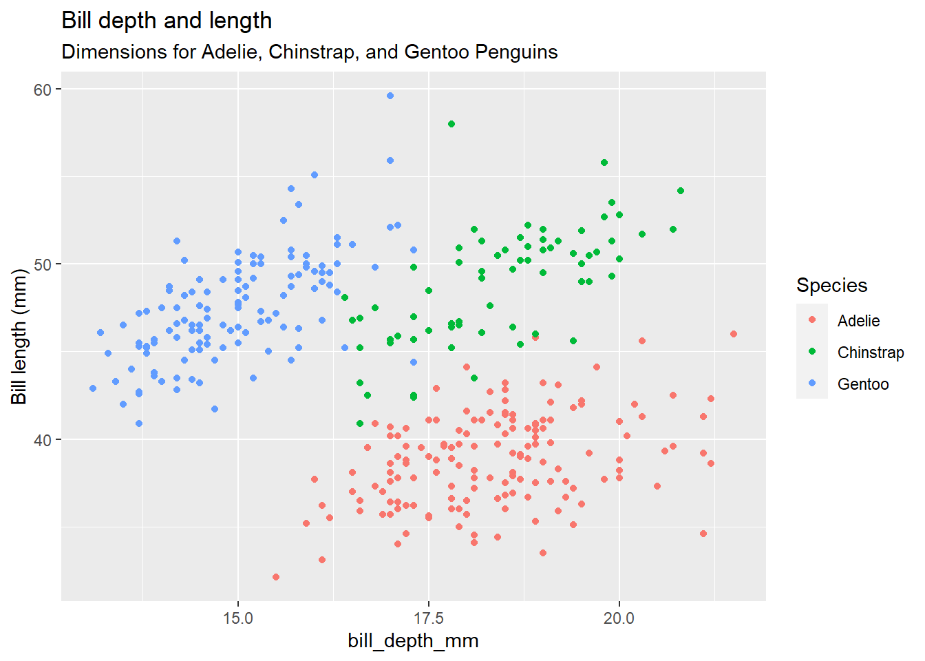

Histogram

Basic Histogram

This is using ggplot2 to create a histogram for the data frame null_distn with the x parameter being the quantiative variable prop(ortion).

null_distn %>% ggplot(aes(x = prop)) +
  geom_histogram(bins = 30, color = "white")

Example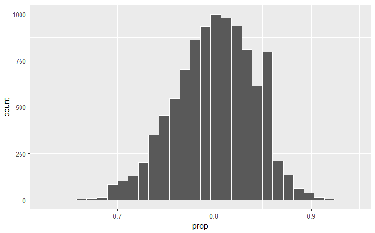
### Histogram showing p-values two-tail test {-}
Recall that the p-value for a two-tail test is the area below/to the left of; and the area above/to the right of our test data point, here 0.73 versus our Null of 0.8.

library(tidyverse)
p_hat <- 73/100
dist <- 0.8 - p_hat
null_distn %>% ggplot(aes(x = prop)) +
  geom_histogram(bins = 30, color = "white") +
  geom_vline(color = "red", xintercept = 0.8 + dist) +
  geom_vline(color = "red", xintercept = p_hat)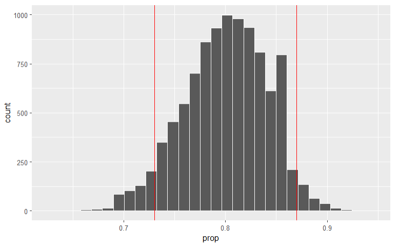

Bar plot

library(ggplot2)
ggplot(data = elec, aes(x = satisfy)) + geom_bar()

This is a barplot with x parameter being a categorical variable named satisfy.
Example 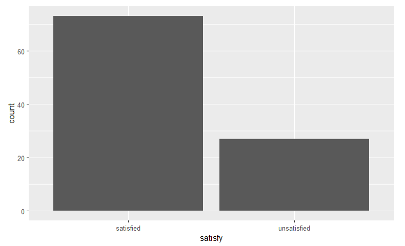We can use this code to create a 100% stacked bar chart and flip the bar chart to horizontal. We have two categorical variables with two and three levels each. party, D or R; opinion, Favor, Indifferent or Oppose.

tax500 %>% ggplot(aes(x = party, fill = opinion)) +
  geom_bar(position = "fill") +
  ylab("Proportion") +
  xlab("Party") +
  ggtitle("Opinion on Tax Bill by Party") +
  coord_flip()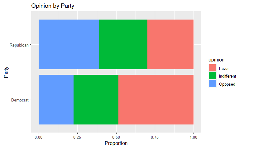

Mosaic plot

A mosaic plot shows using area the proportions of the total count of participants in the survey.

mosaicplot(table(tax500$opinion, tax500$party),
           ylab = "Political Party", 
           xlab = "Tax Reform Bill Opinion",
           main = "Opinion vs Party",
           color = c("lightblue", "pink"))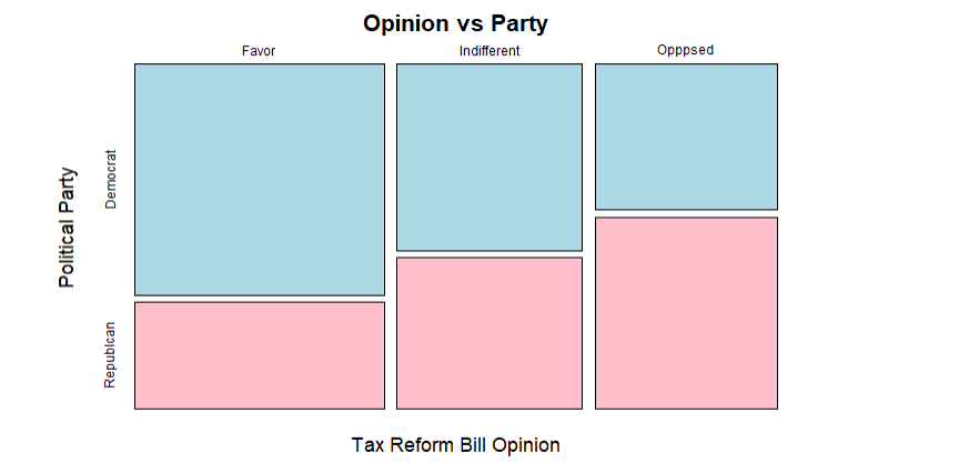

# Save Plots

ggplot(mpg, aes(displ, hwy)) + geom_point()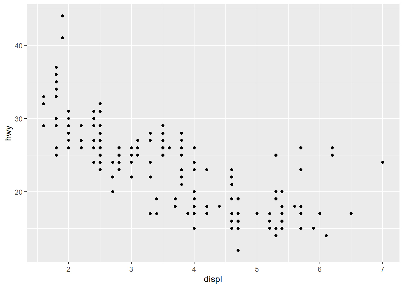

ggsave("my-plot.pdf")
#saves the current plot as `my-plot.pdf`

Code Chunks Used in Labs