Attribution: This lab is an adaptation of materials for Chapter 9 in Modern Dive by Chester Ismay and Albert Y. Kim

Introduction to Hypothesis Tests

Link to Posit Cloud

Log into your Posit Cloud account.
Open the Lab 5 Inference and Confidence Intervals project.
Open the Lab-05-Rehearse2-Worksheet.Rmd.

**IMPORTANT!

Remember to rename this file to include your name in place of “Student-Name” at the top of the page.

Other than entering your name to replace Student Name and changing the date to the current date, do not change anything in the head space.

Load Packages

First load the necessary packages:

CC3

library(tidyverse)
library(infer)

Load Data

For this rehearse we will work with some grade-point-average (GPA) data for college freshman.

The following code chunk will read in the data:

CC4

# When reusing this code chunk in a Remix assignment:
  # Change sat_gpa to the data object name you want to create.
  # Change sat_gpa.csv to the name of your data file.
  # Your data file must be in the data folder.

sat_gpa <- read_csv("data/sat_gpa.csv")

You should see the sat_gpa data object in the Environment as well as a message on the data load process.

Important

For the remainder of this course, the following is the process we will use for all Hypothesis Tests.

Inspect the Data

Hint

There are many ways to inspect your data frame using R. Perhaps the easiest is to just click on the name of the data frame in the Environment so that it opens in the Source Editor window. There it will be displayed as a typical spreadsheet.

The data frame sat_gpa has seven columns and 1000 rows. Each row in this data frame is a student. The columns are the variables which include:

sex - a binary (i.e., two level) categorical variable representing the gender of each student. “Male” or “Female”
sat_verbal - a numerical variable representing the SAT verbal score for the stuent.
sat_math - a numerical variable representing the SAT math score for the student.
sat_Total - a numerical variable representing the total SAT score for the student.
gpa_hs - a binary categorical variable representing the high school GPA range , “low” or “high”.
gpa_fy - a numerical variable representing the GPA of each student their first year of college.

Example 1: Difference in Two Means

Is there a difference in the mean female and male college freshman GPAs?

Important Concept

This test is also known as an Independent Samples Test or as a Two-sample Test. Although the data may come from just one sample, we generally use a categorical variable to identify the groups whose means we want to compare. Importantly, the two groups are independent of one another. Groups are independent when no individual can be in both (or more than one) groups.

In Module 6, we will cover the situation where two groups are dependent: an individual can be in both groups. This test is known as a Paired Samples or a Dependent Samples test. A good example of this is the situation where participants are given a “pre test” before training and a “post test” after training and we want to determine if the training improved the participants’ test scores.

Exploratory data analysis

Examine the data to gather information related to the research question.

Start by looking at the variables of interest.

Visualize the Data

Generate a data visualization that displays the GPAs of the two groups. For comparing means, a box plot is useful.

CC5

ggplot(sat_gpa, aes(x = sex, y = gpa_fy)) + 
  geom_boxplot(fill = "lightblue") + 
  stat_summary(fun = "mean", geom = "point", shape = 23, size = 3, fill = "red") +
  labs(title = "Grade Point Averages for first year college students", 
       x = "Sex", y = "First Year GPA") +
  theme_bw()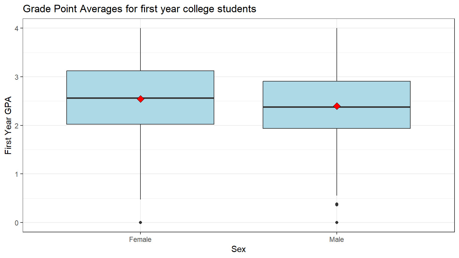

Note: the black bar near the middle of the boxes is the median GPA. The red dot is the mean GPA. You can see that the medians and the means of the two groups are about the same.

Knowledge Check Questions:

Is there a difference in the mean first year GPA’s? Explain why you think this is true.
Your answer here:
Do you think this difference, if any, is large enough to be meaningful? Why do you think this?
Your answer here:

Calculate Means

Calculate the mean FY GPA score for each gender, using the group_by and summarize function from the dplyr package. (Note: the dplyr package is included in the tidyverse package previously loaded.) Then store the results in a new data object named means.

CC6

means <- sat_gpa %>% 
  group_by(sex) %>% 
  summarize(gpa_fy = mean(gpa_fy))

#print the two means
means

## # A tibble: 2 × 2
##   sex    gpa_fy
##   <chr>   <dbl>
## 1 Female   2.54
## 2 Male     2.40

Note: because we did not include code to specify the order of the two levels of the variable sex, R takes them in alphabetical order, i.e. female and then male.

Although we will calculate the difference in the Downey Infer method, we can take a peek at it using a simple code chunk.

CC7

# Calculate the difference in means
mean_difference <- diff(means$gpa_fy)

# Print the mean difference
print(mean_difference)

## [1] -0.1485209

State the Null and Alternative hypotheses

We will now test the Null hypothesis that there’s no difference in mean first year GPA between the genders at the population level.

Ho: The mean FY GPA of females is equal to the mean FY GPA of males.
Ha: The mean FY GPA of females is not equal to the mean FY GPA of males.

Or expressed as a difference:

Ho: The mean FY GPA of females minus the mean FY GPA of males is equal to 0.
Ha: The mean FY GPA of females minus the mean FY GPA of males is not equal to 0.

A more common method of stating the Null and Alternative for this type of problem:

Ho: There is no difference in the mean FY GPA of females and the mean FY GPA of males.
Ha: There is a difference in the mean FY GPA of females and the mean FY GPA of males.

Specify the level of significance (alpha)

We will use the “standard” value of 5% for significance level for this analysis.

Test the hypothesis - Downey Method

Here’s how we use the Downey method with infer package to conduct this hypothesis test:

Step 1: Calculate the observed statistic

Calculate the observed difference delta and store the results in a new data object called delta_obs.

In this example, we are comparing two means, so the observed statistic will be the difference in the means of the two groups using the sample data.

In the next code chunk, we use the specify verb by telling R which variable is the response variable, the numerical variable, and which is the explanatory variable, the categorical variable.

We then use the calculate verb and find the test statistic we want. Here we use the diff in meansstatistic which is the difference in the Female and Male mean gpas.

We can use the order = c() function to specify the order of the two levels of the categorical variable. If we do not specify an order, R will use alphabetical order based on the first letter of the variable names.

Important!

The comments, which are preceded by a hash #, in the following code blocks are intended for use when you reuse them in a Remix assignment. Do not make changes in the code blocks when working on the Rehearse. Just copy/paste/run as normal when in a Rehearse.

CC8

# When reusing this code chunk in a Remix assignment: 
 # The `delta_obs` data object name should not be changed.
 # Change `sat_gpa` to your data set name.
 # change `gpa_fy` to your numerical variable.
 # Change `sex` to your categorical variable.
 # Change "Female" and "Male" to your categorical variable levels.

delta_obs <- sat_gpa %>% 
  specify(gpa_fy ~ sex) %>% 
  calculate(stat = "diff in means", order = c("Female", "Male"))

# Print out the results
delta_obs

## Response: gpa_fy (numeric)
## Explanatory: sex (factor)
## # A tibble: 1 × 1
##    stat
##   <dbl>
## 1 0.149

Step 2: Generate the Null Distribution

Generate the null distribution of the delta test statistic.

This step involves generating simulated values of the difference in means as if we lived in a world where there’s no difference between the two groups of students.

We do this by hypothesizing a null of “independence”’

Going back to the idea of permutation, and tactile sampling, this is akin to shuffling the GPA scores between male and female labels (i.e. removing the structure to the data) just as we could have done with index cards, pennies, or marbles.

We also calculate the delta between male and females under the Null Hypothesis that there is no difference in mean First Year GPA between females and males.

CC9

# When reusing this codein a Remix assignment: 
 # The `null_dist` data object name should not be changed.
 # Change `sat_gpa` to your data set name.
 # Change `gpa_fy` to your numerical variable.
 # Change `sex` to your categorical variable.
 # Change "Female" and "Male" to the levels of your categorical variable.
 # Do not change anything else.

# set seed for reproducible results
set.seed(123)

null_dist <- sat_gpa %>% 
  specify(gpa_fy ~ sex) %>% 
  hypothesize(null = "independence") %>% 
  generate(reps = 1000, type = "permute") %>%
  calculate(stat = "diff in means", order = c("Female", "Male")) 

# Print first 5 rows
null_dist %>% 
  slice(1:5)

## Response: gpa_fy (numeric)
## Explanatory: sex (factor)
## Null Hypothesis: independence
## # A tibble: 5 × 2
##   replicate     stat
##       <int>    <dbl>
## 1         1 -0.00460
## 2         2 -0.0104 
## 3         3 -0.0612 
## 4         4  0.0132 
## 5         5 -0.0249

Questions:

What was the size of the “shuffled” (permuted) sample in each run? Hint: how many rows were in the original data file?
Your answer here:
How many times did we “shuffle” (permute) the sample? Hint: How many rows are in the `null_dist` data object?
Your answer here:

Step 3: Visualize the Null and the “Delta”

Visualize how the observed difference delta_obs compares to the null distribution of delta.

The following code chunk plots the delta values we calculated for each of the different “shuffled” replicates.

This is the null distribution of delta.

The red line shows the observed difference between male and female scores in the data (-0.1485209) from step 1. This is the value of delta_obs from CC8.

Because we are interested in whether there is a difference in mean FY GPA of females and males that is either negative or positive, we need to look at both ends of the distribution, i.e. both directions.

CC10

# When reusing this code chunk in a Remix assignment, edit only
  # the axis labels, 
  # the title, 
  # and the subtitle. 

visualize(null_dist) +
  shade_p_value(obs_stat = delta_obs, direction = "both") +
  labs(x = "Difference in mean First Year GPA for females and males", y = "Count",
       title = "Null distribution of differences in female and male First Year GPAs",
       subtitle = "Actual difference observed (delta_obs) in the data is marked in red"
       ) +
  theme_bw()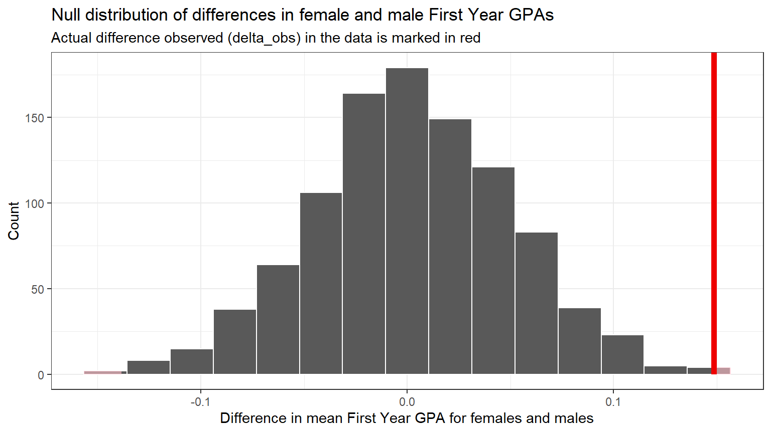

Note that zero is the center of this null distribution because we assumed there is no difference in the two means.

The Null hypothesis is that there is no difference (i.e. 0) between females and males in the first year GPA score.

In the permutations, zero was the most common difference, because observed GPA values were re-assigned to females and males at random. Differences as large as approximately +0.1 and -0.1 occurred, but much less frequently, because they are just not as likely when structure (relationship) is removed from the data.

Important concept:

Note that because the red line delta_obs is in an extreme tail of the distribution, it does not occur often in the Null world.

Explain why the conclusion that the delta_obs does not occur often in the Null world is correct.

Your Answer:

Step 4: Calculate the p-value

Don’t recall what a p-value is? Here is a link to an explanation in one of the assigned readings if you need a refresh 1.3.2 p-value and statistical significance

Using the null_dist data object, we can calculate the p-value from the difference observed in the original data in delta_obs.

CC11

# When reusing this code chunk in a Remix assignment, no changes are needed.

p_value <- null_dist %>% 
  get_pvalue(obs_stat = delta_obs, direction = "both") 

p_value

## # A tibble: 1 × 1
##   p_value
##     <dbl>
## 1   0.002

Remember, your answer may differ due to random chance unless you use the same set.seed value of 123 in CC9 above.

Important

If your p-value is stated as 0, it just means that the probability is very, very small. It is impossible to have a p-value of exactly 0. Accepted practice is to report “p-value < 0.001” when the calculated p-value appears to be 0.

Here, the p-value is shown to be 0.002, which is very small.

This result indicates that there is a 0.002 or 0.2% chance that we would see a difference of 0.149 (or more) in GPA scores between females and males if in fact there was truly no difference between the sexes in first year GPA scores in the population.

Note that we use p_value as the data object name for the “p-value”. This is necessary because R would assume the use of “p-value” in code to be “p minus value” which would cause an error.

Step 5: Decide if delta_obs is statistically significant

Compare the p-value with the significance level alpha. If the p-value is less than alpha, the Null hypothesis must be rejected.

In this example, the significance level alpha was set at 5% or 0.05.

CC12

# When reusing this code chunk in a Remix assignment:
 # Replace the value for alpha with your significance level. 
 # No other changes are needed.

alpha <- 0.05 

if(p_value < alpha){ 
  print("Reject the Null Hypothesis")
} else { 
    print("Fail to reject the Null Hypothesis") 
}

## [1] "Reject the Null Hypothesis"

Question:

If the p-value is greater than the significance level (alpha), statisticians state the result of the analysis is “Fail to reject the Null Hypothesis” instead of declaring the Null Hypothesis to be true.

Question

Explain why it is technically incorrect to state that the Null Hypothesis is true when the p-value is greater than alpha?

Your answer here:

Results and Conclusions

Here is one way to write up the results of this hypothesis test:

The mean GPA scores for females in our sample 2.59 was greater than that of males 2.39. This difference was statistically significant at alpha = 0.05, (p = 0.002).

Given this, Reject the Null hypothesis and conclude that females have higher first year GPAs than males at the population level.

Confidence interval method

Another way to test the Null hypothesis is to calculate a confidence interval surrounding the observed difference.

The following code will allow us to calculate a 95% confidence interval for the difference between mean GPA scores for females and males. A new data object ci_diff is used to hold the results.

CC13

# When reusing this code chunk in a Remix assignment:
 # Do not change the name `ci_diff`
 # Change `sat_gpa` to your data set:
 # Change `gpa_fy` to your numerical variable.
 # Change `sex` to your categorical variable.
 # Change "Female" and "Male" to the levels in your variable.

# Set seed to make the results reproducible.
set.seed(123)

ci_diff <- sat_gpa %>% 
   specify(gpa_fy ~ sex) %>%
   generate(reps = 1000, type="bootstrap") %>% 
   calculate(stat = "diff in means", order = c("Female", "Male")) %>% 
   get_confidence_interval(level = 0.95)

#display the CI
ci_diff

## # A tibble: 1 × 2
##   lower_ci upper_ci
##      <dbl>    <dbl>
## 1   0.0634    0.247

The Null difference of 0 does not fall within the bounds of the confidence interval. That indicates the Null hypothesis of no difference must be rejected.

Traditional Method

Although we recommend the use of the Downey/Infer method in this course, you should be aware that the traditional t-test can be used to perform a test of hypothesis.

Although it appears that many of the above Downey/Infer steps can be done with one line of code, this method only can be used if a slew of assumptions like normality and equal variance of the groups are met. Additional tests to verify that the assumptions are met must be conducted before the results can be used. Check assumptions and tests here.

CC14

# When reusing this code chunk in a Remix assignment:
 # Change gpa_fy to your numerical variable.
 # Change sex to your categorical variable.
 # Change sat_gpa to your data set

t.test(gpa_fy ~ sex, var.equal = TRUE, data = sat_gpa)

## 
##  Two Sample t-test
## 
## data:  gpa_fy by sex
## t = 3.1828, df = 998, p-value = 0.001504
## alternative hypothesis: true difference in means between group Female and group Male is not equal to 0
## 95 percent confidence interval:
##  0.05695029 0.24009148
## sample estimates:
## mean in group Female   mean in group Male 
##             2.544587             2.396066

By inspection, you should notice the results of the two methods are relatively similar. Both have a very small p-value and both have about the same upper and lower limits for the 95% confidence interval.

Unlike in the Downey method where we can specify the order, the traditional t-test uses alphabetical order when calculating the difference between the two levels of the categorical variable. If you specified a different order in the Downey code, you will see the CI is reversed.

Example 2: Test for Correlation

Is there a relationship between a student’s total SAT score and their first year GPA?

In this question, we are interested in knowing if a student’s total SAT score is predictive of their GPA in their first year in college.

We have two numeric variables, so we can use a test for correlation similar to what we did in Module 4 Rehearse 1.

For this analysis, sat_total is the “predictor” or explanatory variable, and gpa_fy is the response variable.

Exploratory data analysis

Examine the data to gather information related to the research question.

Start by looking at the variables of interest.

Visualize the Data

Generate a data visualization that displays the SAT Total scores and the first year GPAs. We can use the scatter/line plot we created in Lab 4 Rehearse 1 in CC3.

CC15

# When reusing this code chunk in a Remix assignment:
 # Change the sat_gpa to your data set.
 # Change sat_total to  one of your numerical variables.
 # Change gpa_fy to your second numerical variable

ggplot(sat_gpa, aes(x=sat_total,y=gpa_fy))+
  # plot the data pairs as points
  geom_point()+
  # add a "best fit" linear trend line to show the slope
  geom_smooth(method=lm, se=FALSE) +
  theme_bw()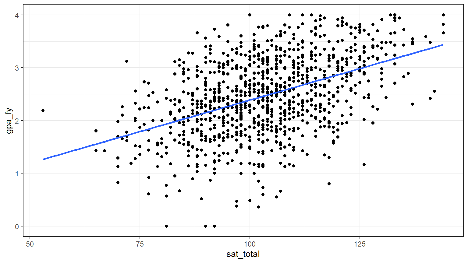

From inspection of the chart, it appears that as the sat_total increases, so does the gpa_fy. But is that relationship just due to chance or is there really a positive correlation?

State the Null and Alternative hypotheses

Ho: There is no relationship between SAT total scores and students’ first year college GPA.
Ha: There is a relationship between SAT total scores and students’ first year college GPA.

Specify the level of significance (alpha)

We will use the “standard” value of 5% for significance level for this analysis.

Test the hypothesis - Downey Method

Step 1: Calculate the observed test statistic

For this analysis, our observed test statistic is the correlation coefficient r between the mean total SAT scores and first year college GPAs. Though it is not really a “difference” per se, we will continue to use Downey’s delta in our code for consistency.

CC16

# When reusing this code chunk in a Remix assignment: 
 # The `delta_obs` data object name should not be changed.
 # Change `sat_gpa` to your data set name.
 # Change `gpa_fy` to your 1st numerical variable.
 # Change `sat_total` to your 2nd numerical variable.

delta_obs <- sat_gpa %>% 
  specify(gpa_fy ~ sat_total) %>% 
  calculate(stat = "correlation")

# Print the correlation r observed in the sample
delta_obs

## Response: gpa_fy (numeric)
## Explanatory: sat_total (numeric)
## # A tibble: 1 × 1
##    stat
##   <dbl>
## 1 0.460

Step 2: Generate the Null Distribution

Generate the null distribution of the correlation coefficient.

Here you need to generate simulated values as if we lived in a world where there’s no relationship between total SAT scores and a student’s first year college GPA. We modle that by assuming the two variables are independent.

CC17

# When reusing this code in a Remix assignment:
 # The `null_dist` data object name should not be changed.
 # Change `sat_gpa` to your data set name.
 # Change `gpa_fy` to your 1st numerical variable.
 # Change `sat_total` to your 2nd numerical variable.

#set seed for reproducibilty
set.seed(123)

null_dist <- sat_gpa %>% 
  specify(gpa_fy ~ sat_total) %>% 
  hypothesize(null = "independence") %>% 
  generate(reps = 1000, type = 'permute') %>%
  calculate(stat = "correlation")

Step 3: Visualize the Null and the “Delta”

Visualize how the observed difference compares to the null distribution of delta, the test statistic which is the correlation coefficient r.

This code will generate a histogram of the null distribution of delta with a vertical red line showing the observed correlation r (delta_obs).

CC18

# When reusing this code chunk in a Remix assignment, edit only
  # the axis labels, 
  # the title, 
  # and the subtitle. 

visualize(null_dist) +
  shade_p_value(obs_stat = delta_obs, direction = "both") +
  labs(x = "Correlation coefficient r", y = "Count",
       title = "Null distribution of correlations between SAT Total scores and students first year GPAs",
      subtitle = "Actual correlation observed in the sample data is marked in red") +
  theme_bw()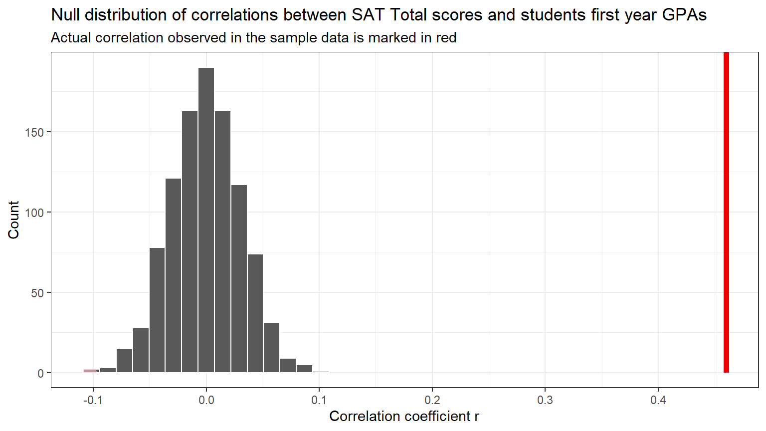

Step 4: Calculate the p-value

CC19

# When reusing this code chunk in a Remix assignment, no changes are needed.
# calculate the p-value and assign it to the `p_value` data object.

p_value <- null_dist %>% 
  get_pvalue(obs_stat = delta_obs, direction = "both") 

p_value

## # A tibble: 1 × 1
##   p_value
##     <dbl>
## 1       0

Step 5: Decide if delta_obs is statistically significant

Compare the p-value with the significance level alpha. If the p-value is less than alpha, the Null hypothesis must be rejected.

In this example, the significance level alpha was set at 5% or 0.05.

CC20

# When reusing this code chunk in a Remix assignment:
 # Replace the value for alpha with your significance level. 
 # No other changes are needed.

alpha <- 0.05 

if(p_value < alpha){ 
  print("Reject the Null Hypothesis")
} else { 
    print("Fail to reject the Null Hypothesis") 
}

## [1] "Reject the Null Hypothesis"

Important

Remember that a p-value cannot be exactly 0. The “0” here just means that the p-value is very small. Best practice is to report this p-value as “p < 0.01.”

Results & Conclusions

Write up the results & conclusions for this hypothesis test.

Answer: There is a moderate positive correlation between a student’s total SAT score and their first year GPA, r = 0.46. This correlation is statistically significant at alpha = 0.05, (p = < 0.01).

Given these results, reject the Null hypothesis and conclude that there is a relationship between a student’s total SAT score and their first year college GPA at the population level.

Confidence Interval

Calculate a confidence interval for the difference in total SAT scores for students with high and low high-school GPA scores.

Note that you should use whatever order you chose above…i.e. order = c("low", "high") or order = c("high", "low").

If you reverse the order, the values of the CI end points will be reversed.

CC21

# When reusing this code chunkin a Remix assignment:
 # Do not change the name `ci_diff`
 # Change `sat_gpa` to your data set:
 # Change `gpa_fy` to your 1st numerical variable.
 # Change `sat_total` to your 2nd numerical variable.

# set seed to make results reproducible
set.seed(123)

ci_diff <- sat_gpa %>% 
  specify(gpa_fy ~ sat_total) %>%
  generate(reps = 1000, type="bootstrap") %>% 
  calculate(stat = "correlation") %>% 
  get_confidence_interval(level = 0.95)

# display the confidence interval around the correlation coefficient
ci_diff

## # A tibble: 1 × 2
##   lower_ci upper_ci
##      <dbl>    <dbl>
## 1    0.409    0.505

As for Question 2, the Null hypothesis value of 0 is not contained in the interval from 0.409 to 0.505. Thus, the Null must be rejected.

This is the same conclusion as before.

Traditional Method

Use a traditional correlation test to determine if there is a statistically significant correlation between a student’s total SAT scores and their first year college GPA at the population level.

CC22

# When reusing this code chunk in a Remix assignment:
 # Do not change the name of the data object correlation_test.
 # Change sat_gpa to your data set.
 # Change sat_total to a numerical variable.
 # Change sat_gpa to your data set.
 # Change gpa_fy to a numerical variable.

# Perform the correlation test
correlation_test <- cor.test(sat_gpa$sat_total, sat_gpa$gpa_fy)

# Print the results
print(correlation_test)

## 
##  Pearson's product-moment correlation
## 
## data:  sat_gpa$sat_total and sat_gpa$gpa_fy
## t = 16.379, df = 998, p-value < 2.2e-16
## alternative hypothesis: true correlation is not equal to 0
## 95 percent confidence interval:
##  0.4099866 0.5077848
## sample estimates:
##      cor 
## 0.460281

Again, the traditional correlation test produces essentially the same results but the results should not be used until the required assumptions are checked and verified.

Lab Assignment Submission

Important

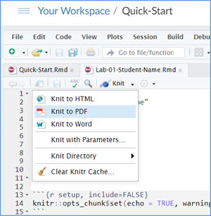
When you are ready to create your final lab report, save the Lab-05-Rehearse2-Worksheet.Rmd lab file and then Knit it to PDF or Word to make a reproducible file. This image shows you how to select the knit document file type.

Note that if you have difficulty getting the documents to Knit to either Word or PDF, and you cannot fix it, just save the completed worksheet and submit your .Rmd file for partial credit.

Ask your instructor via course email to help you sort out the issues if you have time.

Submit your file in the M5.2 Lab 5 Rehearse(s): Estimation and Confidence Intervals assignment area.

The Lab 5 Inference: Estimation and Confidence Intervals Grading Rubric will be used.

Previous: Lab 5 Rehearse 1

Next: Lab 5 Remix

Lab Manual Home Page

This work was created by Dawn Wright and is licensed under a Creative Commons Attribution-ShareAlike 4.0 International License.

Version 2.3, date 4/6/24

Last Compiled 2024-04-09

Lab 5 Rehearse 2