Lab 7 Rehearse 2
Samples with Multiple Proportions
Lab 7 Rehearse 2
Link to Posit Cloud
- Log into your Posit Cloud account.
- Open the Lab 7 Hypothesis Tests 2 workspace.
- Open the Lab7-Rehearse2-Worksheet.Rmd.
Note that you will do all your work for this rehearse in the Lab7-Rehearse2-Worksheet.Rmd.
 IMPORTANT!
Remember to edit this file to include your name in place of “Student-Name” at the top of the page.
Other than entering your name to replace Student Name and changing the date to the current date, do not change anything in the head space.
Samples with Multiple Proportions
Introduction
In the first rehearse of module 7, we learned how to compare a single proportion found in one sample to a standard or assumed value. And to compare the single proportions found in two samples to each other.
But what do we do when we have more than two proportions in a sample to compare?
Of course, we have a test for that situation. And it is an oldie but a goodie.
In fact, the test we use is one of the oldest hypothesis tests which was invented by Karl Pearson around the turn of the century, the goodness of fit test which uses the Chi-squared distribution instead of the normal or t distributions we have previously discussed.
But don’t worry.
We are not going to get deep into theory here, but just let R do the background work for us again.
One Categorical Variable: Goodness of Fit Test

Important concept: When we are interested in one categorical variable which has more than two levels, we can use a Chi-square Goodness of Fit test.
A particular brand of candy-coated chocolate comes in five different colors: brown, coffee, green, orange, and yellow. The manufacturer of the candy says the candies colors are distributed in the following proportions in each package: brown - 40%, coffee - 10%, green - 10%, orange - 20%, and yellow - 20%.
A random sample from bags of candy at a drug store was taken. The bag selected had 102 pieces of this candy.
Does this random sample provide sufficient evidence against the manufacturer’s claimed distribution of colors that we can conclude the actual distribution of the proportions of colors is different?
We will answer this question using the Downey-Infer process.
Important Concept: In this type of problem, we are comparing a distribution of proportions (parts of a whole) in our sample to the distribution of proportions planned or previously found.
Load Packages
First load the necessary packages:
 CC1
CC1
library(tidyverse)
library(infer)
Load the data
The following code chunk will read in the data which is in the Lab 7 project data folder:
CC2
# This code will load the required CSV data file from the workspace /data folder.

candies <- read.csv("./data/candies3.csv")

#using the glimpse function to display the data object
glimpse(candies)
## Rows: 102
## Columns: 1
## $ actual <chr> "brown", "brown", "brown", "brown", "brown", "brown", "brown", …Inspect the Data
You should see the candies data object in the
Environment. Remember you can click on the name and it will open in the
Source Editor window.
There is one categorical variable, actual, with 102
observations in the sample.
Exploratory data analysis
Find unique colors of candy
We can display the levels of the categorical variable
actualusing the following code. By “levels” we mean unique
values of actual in the column of data.
CC3
# Display the levels of the categorical variable 'color'

unique(candies$actual)
## [1] "brown" "green" "coffee" "orange" "yellow"So, we have do have the five standard colors of candy in the sample.
Visualize the data
In the following code chunk, we create a bar chart to display the
count of each of the colors in the sample dataset
candies.
CC4
ggplot(data = candies, aes(x = actual, fill = actual)) +
  geom_bar() +
  theme_bw()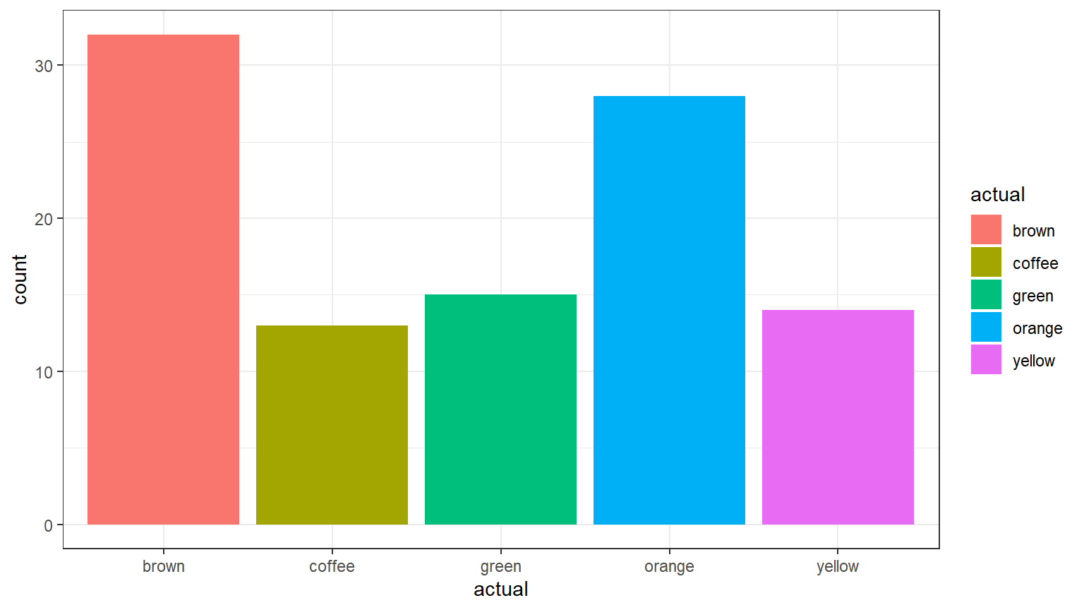
Find the counts
We can find the counts of the number of candy pieces of each color in the sample.
CC5
# This code creates a table that summarizes the numbers of each color.
color_count <- table(candies$actual)
# This displays the table.
color_count
##
## brown coffee green orange yellow
## 32 13 15 28 14Find the proportions
Because we are interested in the distribution of proportions of the colors in the sample, we also calculate the proportions of each color in the sample.
CC6
obs_prop <- prop.table(table(candies$actual))
#display the table of proportions of the candy colors in the sample.
obs_prop
##
## brown coffee green orange yellow
## 0.3137255 0.1274510 0.1470588 0.2745098 0.1372549
Question: This is the distribution of the proportions of the colors “planned” by the manufacturer: brown - 40%, coffee - 10%, green - 10%, orange - 20%, and yellow - 20%.
Are there differences in the planned and the observed proportions?
Your answer here:
Question: Make a guess: are these differences between the planned and observed proportions statistically significant?
Your answer here:
State the Null and Alternative hypotheses
Null hypothesis Ho: The true proportions in the sample match what the manufacturer states is the planned proportions: brown - 40%, coffee - 10%, green - 10%, orange = 20%, and yellow - 20%.
Alternative hypothesis Ha: The distribution of candy proportions observed in the sample differs from what the manufacturer states.
Specify the level of significance (alpha)
It’s important to set the significance level “alpha” before starting the testing using the data.
Let’s set the significance level at 5% ( i.e., 0.05) here because nothing too serious will happen if we are wrong. (we are not going to publish our results!)
Test the hypothesis - Downey Method
Here’s how we use the Downey method with
infer package to conduct this hypothesis test:
Step 1: Calculate the observed statistic
Calculate the observed statistic delta and
store the results in a new data object called
delta_obs.
We do this by comparing the observed proportions in the sample against the hypothesized (planned) proportions.
Note that we use a “point” null even though we have five values - they are all point values.
Important Concept: The sum of the planned proportions values add up to exactly 1 in the ‘hypothesize’ step in the analysis. Be careful of rounding.
We use the Chi-square statistic for our difference Delta. For our purposes, don’t worry too much about just what the Chi-square is. It is just a type of number we can calculate from the data, just as we previously calculated the mean.
CC7
delta_obs <- candies %>%
   specify(response = actual) %>%
# use the planned values here, not the observed proportions
  hypothesize(null = "point",
              p = c("coffee" = 0.1,
                    "brown" = 0.4,
                    "yellow" = 0.2,
                    "orange" = 0.2,
                    "green" = 0.1)) %>%
  calculate(stat = "Chisq")

#Display the results
delta_obs
## Response: actual (factor)
## Null Hypothesis: point
## # A tibble: 1 × 1
## stat
## <dbl>
## 1 9.76Our observed difference Delta equals a Chi-square value of 9.7647.
Step 2: Generate the Null Distribution
Generate the null distribution of the difference delta.

For an explanation of the generate function type = draw,
see here.
CC8
#set seed for reproducible results
set.seed(123)

#create the null distribution
null_dist <- candies %>%
   specify(response = actual) %>%
  hypothesize(null = "point",
              p = c("brown" = 0.4,
                    "coffee" = 0.1,
                    "green" = 0.1,
                    "orange" = 0.2,
                    "yellow" = 0.2)) %>%
  generate(reps = 1000, type = "draw") %>%
  calculate(stat = "Chisq")

null_dist
## Response: actual (factor)
## Null Hypothesis: point
## # A tibble: 1,000 × 2
## replicate stat
## <int> <dbl>
## 1 1 1.33
## 2 2 1.63
## 3 3 1.43
## 4 4 2.75
## 5 5 2.41
## 6 6 9.76
## 7 7 2.12
## 8 8 0.794
## 9 9 3.44
## 10 10 4.03
## # ℹ 990 more rowsStep 3: Visualize the Null Distribution and the Delta
Visualize how the observed difference delta_obs compares
to the null distribution of delta.
The following plots the delta values we calculated for each of the different “shuffled” replicates. It creates a histogram to show the distribution of the values of delta. This is the null distribution of delta.
The red line shows the observed test statistic which is the value of
delta_obs.
Important Concept: Unlike the difference in means we previously worked with, the Chi-square test is only a right tail or “greater” test.
CC9
#Note the Chi-square test is always a right-tail test
visualize(null_dist) +
  shade_p_value(obs_stat = delta_obs, direction = "greater") +
  theme_bw()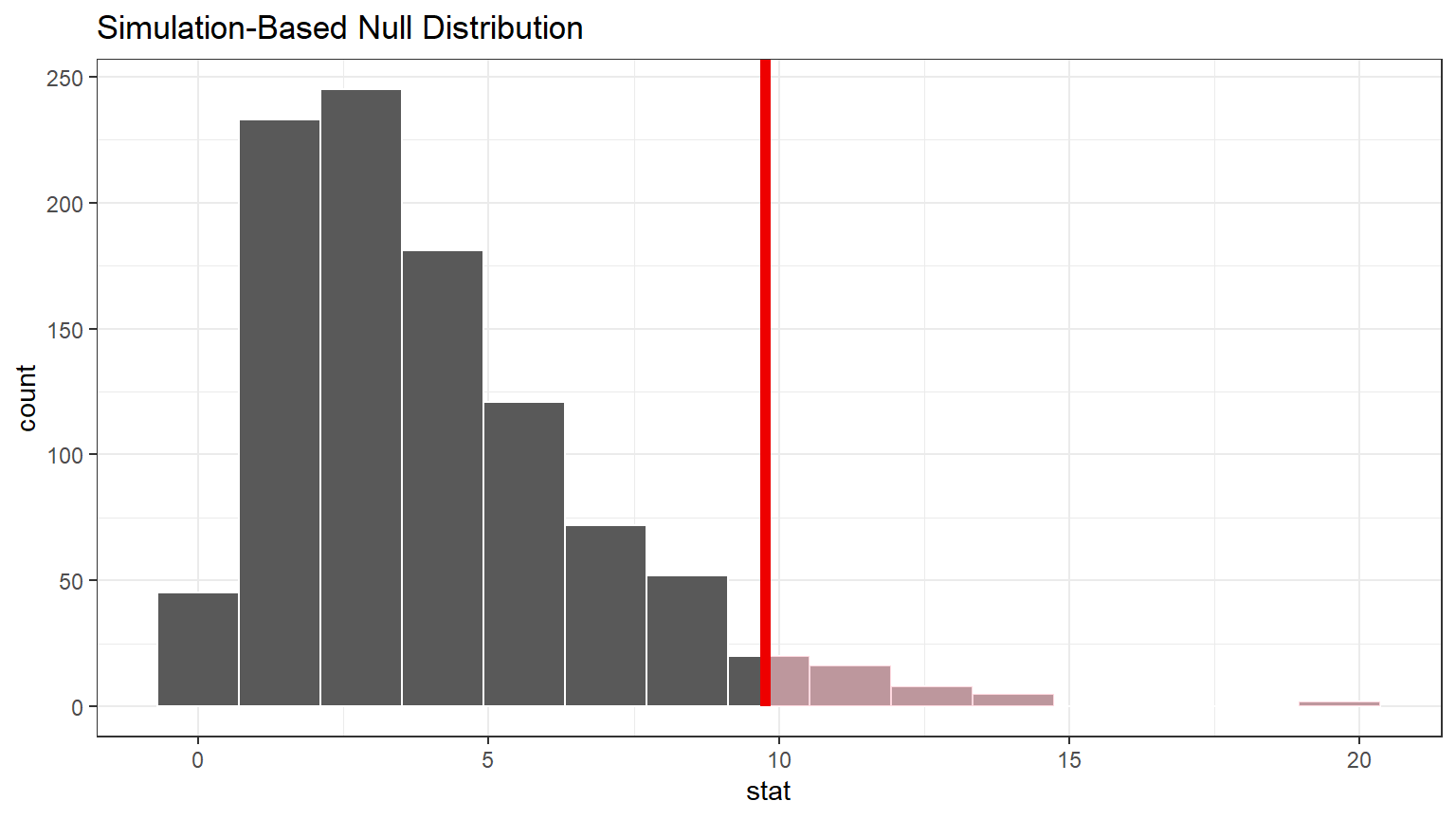
The observed test statistic of 9.76 does not appear to be in the extreme “tail” of the null distribution. But it also is not near the middle of the distribution. This delta_obs may or may not be unusual.
Important concept: Remember that the area of the “pinkish” shaded portion of the distribution represents the probability of getting a value of `delta_obs` as extreme or even more extreme delta - i.e. the p-value.
Step 4: Calculate the p-value
Calculate the p-value (the “pink” area of the histogram beyond
delta_obs).
CC10
p_value <- null_dist %>%
  get_p_value(obs_stat = delta_obs, direction = "greater")

p_value # display the p_value
## # A tibble: 1 × 1
## p_value
## <dbl>
## 1 0.045Step 5: Decide if delta_obs is statistically significant
Compare the p-value with the significance level alpha. If the p-value is less than alpha, the Null hypothesis must be rejected.
CC11
alpha <- 0.05

if(p_value <= alpha){
  print("Reject the Null Hypothesis")
} else {
    print("Fail to reject the Null Hypothesis")
}
## [1] "Reject the Null Hypothesis"Results and Conclusions
Because the p-value of 0.045 is less than the significance level of 0.05, we reject the Null Hypothesis of no difference.
Therefore we conclude that the observed distribution of proportions of candy colors is not the same as the planned distribution of proportions of candy colors.
Calculate confidence interval
The confidence interval approach is not used for Chi-square tests.
Traditional hypothesis test
This is the Chi-square Goodness of Fit test. We use the table function we used in the Exploratory Analysis above to obtain the counts or actual frequencies. Then use the expected proportions in alphabetical order of the names of the levels of the ‘actual’ categorical variable.
CC12
count1 <- table(candies$actual)
trad <- chisq.test(count1, p = c(0.4,0.1,0.1,0.2,0.2))
trad
##
## Chi-squared test for given probabilities
##
## data: count1
## X-squared = 9.7647, df = 4, p-value = 0.04458By inspection, you should notice the results of the two methods are relatively similar.
But to use the traditional (formula-based, theoretical) Chi-square test there are several assumptions which must be checked.
See Assumptions for Traditional Tests
Note: you do not need to actually check the assumptions of the traditional test for this course.
Question: Explain in your own words in a few sentences what the Goodness of Fit test does.
Your Answer here:
Two Categorical Variables: Test for Independence
Recall in Module 4, we looked for a relationship, a correlation, between two quantitative variables, such as height and shoe size. If we have a sufficient sample, we can first make a scatter plot to look for a “trend” in the pattern of dots, the data points. And we can plot a best fit line to help us see the trend more easily. If the line is sloping up from left to right, we have a positive correlation: as the x-variable increases, the y-variable increases. If the line slopes downward from left to right, we have a negative correlation: as x increases, y decreases. And, of course, we can have a situation in which there is no relationship, no obvious trend either way.
We can also look for a relationship between two categorical variables using the Chi-square Test for Independence.
Important concept: We can use the Test for Independence when at least one of the categorical variables has more than two levels.
When both of the two categorical variables of interest have just two levels, use the Test For Two Proportions in Lab 7 Rehearse 1. If the result of that test is that the proportions are different, then the two categorical variables are not independent, but rather are related. And using the Test for Two Proportions when both variables have only two levels also tells us the direction and magnitude of the relationship.
Problem Statement: A random sample of 500 U.S. adults was questioned regarding their political affiliation (democrat or republican) and opinion on a tax reform bill (favor, indifferent, opposed).
Based on this sample, do we have reason to believe that political party and opinion on the bill are related?
Load Packages
First load the necessary packages:
CC13
library(tidyverse)
library(infer)
Load the data
CC14
tax500<- read.csv("./data/tax500.csv")

#using the glimpse function to display the data object
glimpse(tax500)
## Rows: 500
## Columns: 2
## $ party <chr> "Republcan", "Republcan", "Republcan", "Republcan", "Republcan…
## $ opinion <chr> "Favor", "Favor", "Favor", "Favor", "Favor", "Favor", "Favor",…Inspect the Data
Looking at the tax500 data object (either by clicking
once on the name to see it in the Environment; or clicking twice to open
it in the Source Editor window) you should see there are two categorical
variables: party and opinion. And there are
500 observations (rows).
Exploratory data analysis
Let’s find the unique values of the categorical variables:
CC15
# Display the levels of the categorical variable `party`

unique(tax500$party)
## [1] "Republcan" "Democrat" CC16
# Display the levels of the categorical variable `opinion`

unique(tax500$opinion)
## [1] "Favor" "Indifferent" "Opppsed"Thus we have two levels in the party variable and three
in the opinion variable.
Find the counts
We can create a table showing the counts of the two variables with this code.
CC17
# Use the table function to create the table
counts <- table(tax500$opinion, tax500$party)

counts
##
## Democrat Republcan
## Favor 138 64
## Indifferent 83 67
## Opppsed 64 84
This table is called a 3 by 2 contingency table, i.e. 3 rows and 2 columns.
Question: Do you think there is a relationship between the two variables based on looking at the table of counts? Explain why or why not.
Your answer here:
Find the proportions
We can also calculate the proportions in the sample data.
CC18
# Calculate proportions in each column (ie the party affiliation)
# Using the round function to round the values to 3 decimals
proportions <- round(counts / colSums(counts), 3)

# Print the resulting table
proportions
##
## Democrat Republcan
## Favor 0.484 0.298
## Indifferent 0.386 0.235
## Opppsed 0.225 0.391
Question: Do you think there is a relationship between the two variables based on looking at the table of proportions? Explain why or why not.
Your answer here:
Visualize the Data
We will next generate a data visualization that displays the proportions of the opinions of the two groups.
CC19
tax500 %>% ggplot(aes(x = party, fill = opinion)) +
  geom_bar(position = "fill") +
  ylab("Proportion") +
  xlab("Party") +
  ggtitle("Opinion by Party")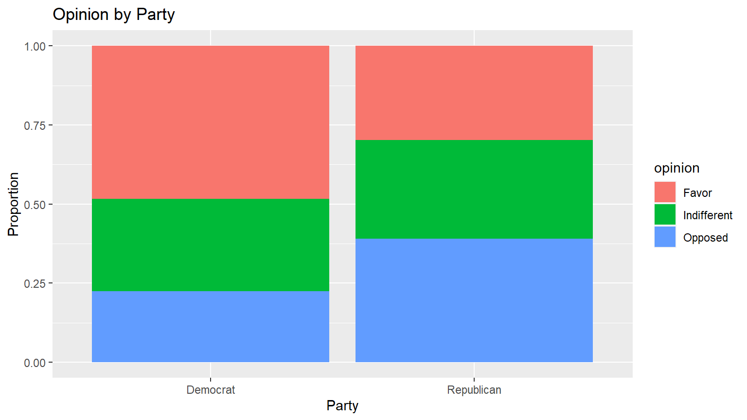
Question: Do you think there is a relationship between the two variables based on looking at the graph? Explain why or why not.
Your answer here:
State the Null and Alternative hypotheses
Null Hypothesis, Ho: There is no relationship between political party and opinion on a tax reform bill.
Alternative Hypothesis, Ha: There is a relationship between political party and opinion on a tax reform bill.
Specify the Significance Level Alpha
Remember it is important to set the significance level “alpha” before starting the analysis.
Let’s set the significance level “alpha” at 5% ( i.e., 0.05) here because nothing too serious will happen if we are wrong.
Test the hypothesis
Step 1: Calculate the observed statistic
We will again be using the Pearson Chi-squared test statistic.
CC20
delta_obs <- tax500 %>%
  specify(formula = party ~ opinion) %>%
  hypothesize(null = "independence") %>%
  calculate(stat = "Chisq")

#display delta_obs
delta_obs
## Response: party (factor)
## Explanatory: opinion (factor)
## Null Hypothesis: indep...
## # A tibble: 1 × 1
## stat
## <dbl>
## 1 22.2Step 2: Generate the Null Distribution
Generate the null distribution of delta.
Here you need to generate simulated values as if we lived in a world where there’s no relationship between a person’s political affiliation and their opinion on the tax bill.
CC21
#set seed for reproducibilty
set.seed(123)

null_dist <- tax500 %>%
  specify(party ~ opinion) %>%
  hypothesize(null = "independence") %>%
  generate(reps = 1000, type = "permute") %>%
  calculate(stat = "Chisq")
For an explanation of the generate function
type = permute, see here.
Step 3: Visualize the Null Distribution and the Delta
CC22
visualize(null_dist) +
  shade_p_value(obs_stat = delta_obs, direction = "greater") +
  theme_bw()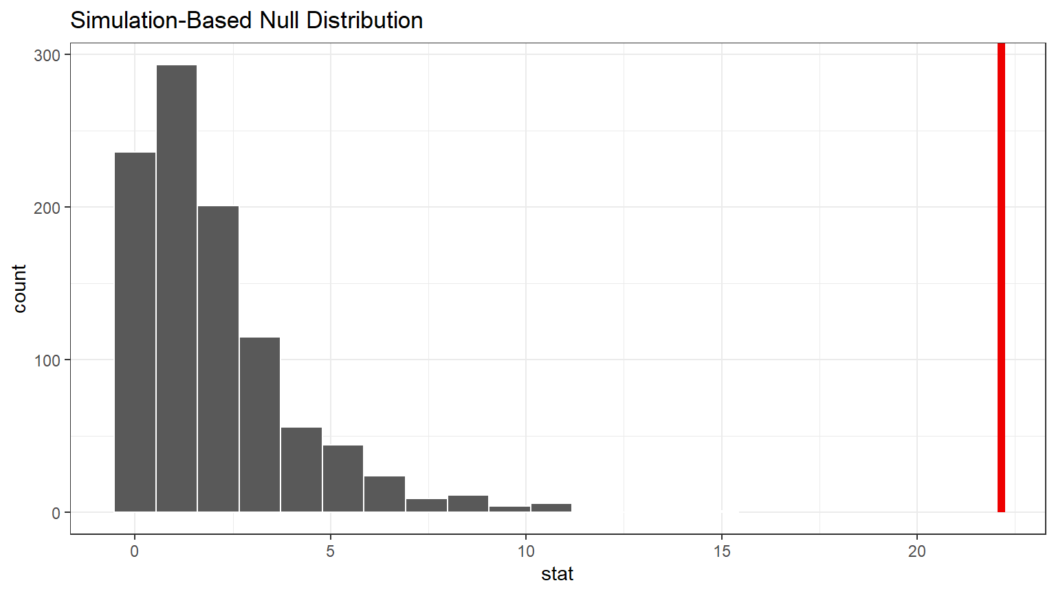
The observed Delta (red line) is far out in the tail of the distribution. This tells us it does not occur often in the Null world.
Question: Do you think there is a relationship between the two variables based on looking at this visualization? Explain why or why not.
Your answer here:
Step 4: Calculate the p-value
CC23
p_value <- null_dist %>%
  get_pvalue(obs_stat = delta_obs, direction = "greater")

p_value
## # A tibble: 1 × 1
## p_value
## <dbl>
## 1 0This very small p-value confirms that the Observed Delta is unusual in the Null world.
Remember that a p-value cannot be exactly 0. Best practice is to report very small p-values like this one as (p < 0.001).
Step 5: Decide if delta_obs is statistically significant
Compare the p-value with the significance level alpha. If the p-value is less than alpha, the Null hypothesis must be rejected.
CC24
alpha <- 0.05

if(p_value <= alpha){
  print("Reject the Null Hypothesis")
} else {
    print("Fail to reject the Null Hypothesis")
}
## [1] "Reject the Null Hypothesis"Results & Conclusions
The observed Chi-square test statistic is 22.15, which falls in the extreme right tail of the distribution. This result is statistically significant at alpha = 0.05, (p = < 0.001).
Based on this sample, we have sufficient evidence that the party and opinion variables are not independent. The respondent’s party affiliation did impact their opinion on the tax bill.
Traditional Method
Use a traditional Chi-square Test for Independence to test the null hypothesis that there is no relationship between political party and opinion on a tax reform bill.
CC25
tax500 %>%
  chisq_test(formula = party ~ opinion)
## # A tibble: 1 × 3
## statistic chisq_df p_value
## <dbl> <int> <dbl>
## 1 22.2 2 0.0000155Note that this p-value is formatted in “scientific notation” which is used for very large and very small numbers. Here, the “e-05” tells us to multiply the 1.547578 times 10 to the -5 power. That will move the decimal point 5 places to the left to give the p-value of 0.0000158.
Again, the traditional test produces essentially the same results but they should not be used until the required assumptions are checked and verified. See Assumptions for Traditional Tests
Question: Explain in your own words in a few sentences what the Test for Independence does.
Your Answer here:
Lab Assignment Submission
Important
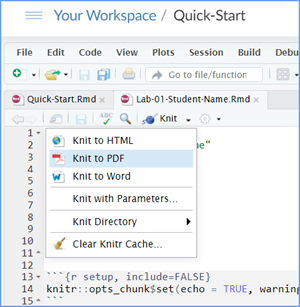
When you are ready to create your final lab report, save the Lab-07-Rehearse2-Worksheet.Rmd lab file and then Knit it to PDF or Word to make a reproducible file. This image shows you how to select the knit document file type.
Note that if you have difficulty getting the documents to Knit to either Word or PDF, and you cannot fix it, just save the completed worksheet and submit your .Rmd file for partial credit.
Submit your file in the Canvas M7.2 Lab 7 Rehearse(s): Hypothesis Tests Part 2 - Proportions assignment area.
The Lab 7 Hypothesis Tests Part 2 Grading Rubric will be used.
Congrats! You have finished Rehearse 2 of Lab 7. Now go to the Remix!


This
work was created by Dawn Wright and is licensed under a
Creative
Commons Attribution-ShareAlike 4.0 International License.
Date 4/4/26
Last Compiled 2026-04-04