Lab 7 Rehearse 1
Comparing One-sample and Two-sample Proportions
Lab 7 Set Up
Posit Cloud Set Up
Just as in previous labs, you will need to follow this link to set up Lab 7 in your Posit Cloud workspace: Link to Set up Lab 7 Hypothesis Tests Part 2 Means
 Important
After you have set up Lab 7 using the link above, do not use that link again.
Instead use this Link to go to Posit Cloud to continue to work on lab 7
RStudio Desktop Setup
Link to download the Lab 7 materials to RStudio Desktop
Note that you will do all your work for this Rehearse 1 in the Lab-7-Rehearse 1 worksheet, so click on that to open it in the Editor window in your RStudio/Posit Cloud Lab 7 workspace.
Introduction to Inference about Proportions
While the terms “1-sample” and “2-sample” might imply multiple sets of data, they actually refer to the context in which proportions are analyzed within a single sample.
In 1-sample proportions, we’re exploring the characteristics or proportions within a single group or population. We investigate and draw inferences about the proportion of successes or events within that single sample, comparing it to a known or hypothesized value.
On the other hand, 2-sample proportions involve comparisons between two different groups or conditions within a single sample. For instance, comparing the proportion of successes or events between two groups (like treatment vs. control, before vs. after, etc.) within the same sample.
Despite the terminology implying multiple samples, both scenarios primarily rely on information derived from a single sample. The distinction lies in how we frame our analysis: either exploring a single group’s proportion or comparing proportions between different subgroups within that same sample. This methodology allows us to infer broader conclusions about populations based on this single set of observed data.

Important Concept: Previously when we were looking at means, we used numerical variables to calculate the means. But sometimes we do use a categorical variable to identify groups whose means we want to compare. In the analysis of proportions, we use categorical variables as our focus.
As we have done in prior modules, we will conduct our analysis using the Downey Method and the Infer package.
One-sample Proportion
Comparing a proportion found in a sample to a standard or claimed value.
Important concept: We use the One-sample proportion test when we have one categorical variable with just two levels.
A large public utility advertises that 80 percent of its over 1,000,000 customers are satisfied with the service they receive. A local politician running for mayor of the city claims that fewer than 80% are satisfied with the utility’s service. To test this claim, the local newspaper surveyed customers, using simple random sampling. 115 people responded to the survey. They found 82 customers said they were satisfied and the remaining 33 were not satisfied.
Based on these findings from the sample, can we reject the politician’s claim that less than 80% of the utility’s customers are satisfied?
Load Packages
First load the necessary packages:
 CC1
CC1
library(tidyverse)
library(infer)
Load the Data
CC2
survey <- read_csv("data/utility_survey2.csv")

#using the glimpse function to display the data object
glimpse(survey)
## Rows: 115
## Columns: 1
## $ satisfied <chr> "yes", "yes", "yes", "no", "yes", "yes", "no", "yes", "yes",…Inspect the Data
In the glimpse, we can see that the survey data object
has 115 rows or observations of the variable satisfied,
which is a categorical variable. We can see “yes” and “no” responses.
But to be sure of how many levels there are we can use the unique
function.
CC3
unique(survey$satisfied)## [1] "yes" "no"This confirms that there are only two levels: yes and no.
Exploratory data analysis
Visualize the data
Because our data is relatively simple, we can use a bar plot to visualize it.
CC4
ggplot(data = survey, aes(x = satisfied, fill = satisfied)) + geom_bar() +
    theme_bw()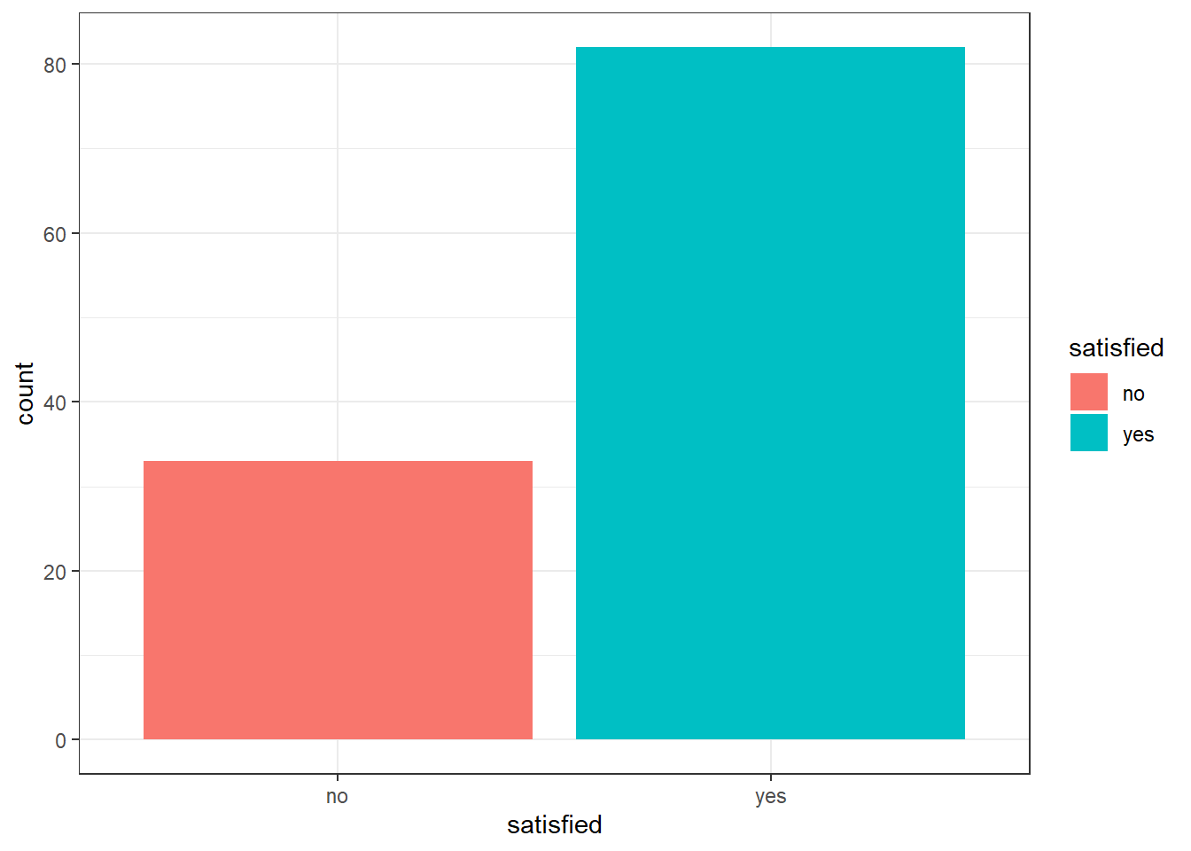
We can see that the “no” column is much smaller than the “yes” column, but we will need more analysis before we can know whether the CEO’s claim is true.
Calculate Proportions
We can use the following code chunk to create a table showing the proportions of “yes” and “no” responses.
CC5
# Create a table with the counts of 'yes' and 'no' survey responses.
 # Then convert to a prop.table with the proportions of 'yes' and 'no'.
 # Then round the proportions to 3 decimal places.
 # Then assign that to the data object 'proportions'.

proportions <- round(prop.table(table(survey$satisfied)),3)

# Print `proportions`
proportions
##
## no yes
## 0.287 0.713So, about 71% of the survey respondents are satisfied. Clearly that is a smaller proportion of satisfied customers than the 80% the utility advertises, but is there enough evidence in this sample to support the politician’s claim that the population proportion of satisfied customers is less than 80%?
State the Null and Alternative hypotheses
Null hypothesis: The proportion of all customers of the large electric utility satisfied with service they receive is equal to or greater than 0.80.
Alternative hypothesis: The proportion of all customers of the large electric utility satisfied with service they receive is less than 0.80.

Question: What is the direction of this hypothesis test?
Your answer:
Question: Explain why we put the politician’s claim as the Alternative Hypothesis?
Your answer:
State the Significance Level
It’s important to set the significance level “alpha” before starting the testing using the data.
Let’s set the significance level at 5% ( i.e., 0.05) here because nothing too serious will happen if we are wrong.
Test the hypothesis - Downey Method
Here’s how we use the Downey method with
infer package to conduct this hypothesis test:
Step 1: Calculate the observed statistic
Calculate the observed statistic and store the results in a new data
object called delta_obs. This is the proportion of “yes” in
the sample data.

Although this observed statistic is not really a difference (a
delta), we continue to use the delta_obs data object name
for consistency with our Downey-Infer process.
Because we are just interested in a single proportion, we only need
to specify our response variable satisfied. The test
statistic we are using is the proportion of “yes” responses. We use the
success = “yes” code to calculate that proportion. We also need
to tell Infer that we want to calculate the proportion statistic using
calculate(stat = “prop”.)
You can find the other available statistics for the calculate() verb here.
CC6
delta_obs <- survey %>%
  specify(response = satisfied, success = "yes") %>%
  calculate(stat = "prop")

delta_obs
## Response: satisfied (factor)
## # A tibble: 1 × 1
## stat
## <dbl>
## 1 0.713Step 2: Generate the Null Distribution
Generate the null distribution of the proportion of satisfied customers. We will hypothesize a Null single “point” proportion value of 0.80.
CC7
set.seed(12)

null_dist <- survey %>%
  specify(response = satisfied, success = "yes") %>%
  hypothesize(null = "point", p = .8) %>%
  generate(reps = 5000, type = "draw") %>%
  calculate(stat = "prop")

null_dist  #display
## Response: satisfied (factor)
## Null Hypothesis: point
## # A tibble: 5,000 × 2
## replicate stat
## <int> <dbl>
## 1 1 0.826
## 2 2 0.791
## 3 3 0.783
## 4 4 0.8
## 5 5 0.826
## 6 6 0.826
## 7 7 0.826
## 8 8 0.861
## 9 9 0.8
## 10 10 0.809
## # ℹ 4,990 more rows
Question: In the code for the test statistic, `delta_obs`, we are using a “point” value for the statistic of 0.80. But the Null hypothesis says ” equal to or greater than 0.80.” Why is just using the point value of 0.80 sufficient to allow us to test the Null Hypothesis?
Your answer:
Step 3: Visualize the Null and the Observed Statistic
CC8
visualize(null_dist) +
  shade_p_value(obs_stat = delta_obs, direction = "less") +
  labs(x = "Proportion of Yes", y = "Count",
     title = "Null distribution of proportion of Yes responses",
     subtitle = "Proportion observed in the sample (delta_obs) data is marked in red"
     ) +
  theme_light()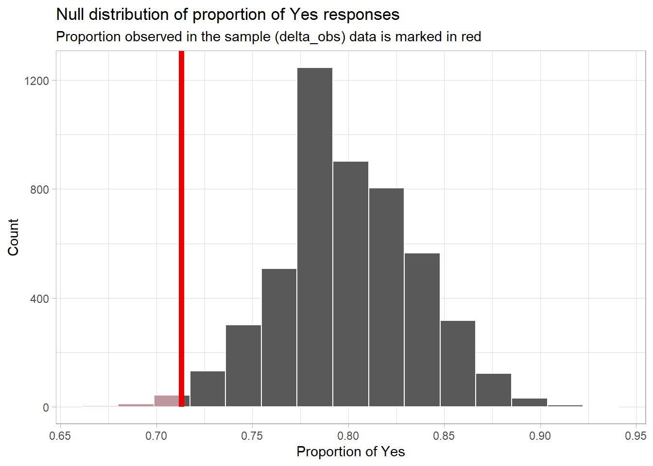
Question: In the code for the visualization, we set the direction to “less”. Explain why this is appropriate for this visualization.
Your answer:
Question: Is the observed sample proportion (delta_obs)
unlikely to happen often in the Null world? Support your answer by
explaining why you think this?
Your answer here:
Step 4: Calculate the p-value
Calculate the p-value - the “area” under the curve (the distribution
of proportions in the Null world ( in null_dist) beyond the
observed sample proportion delta_obs.
CC9
p_value <- null_dist %>%
  get_p_value(obs_stat = delta_obs, direction = "less")


p_value  #print p_value
## # A tibble: 1 × 1
## p_value
## <dbl>
## 1 0.012Step 5: Decide if delta_obs is statistically significant
Compare the p-value with the significance level alpha. If the p-value is less than alpha, the Null hypothesis must be rejected.
CC10
alpha <- 0.05

if(p_value <= alpha){
  print("Reject the Null Hypothesis")
} else {
    print("Fail to reject the Null Hypothesis")
}
## [1] "Reject the Null Hypothesis"The p-value of 0.012 is less than our alpha of 0.05, so we must reject the Null Hypothesis.
Results and Conclusions
We conclude that the proportion of the customers who are satisfied is less then the 80% advertised by the utility. This result supports the politician’s claim.
Calculate confidence interval
The following code chunk creates a 95th percentile confidence interval around the population proportion of satisfied customers using the bootstrap method. For our purposes, we are just using a conventional non-directional confidence interval. A more nuanced result could be found using a directional CI, but that is beyond the scope of our course.
CC11
set.seed(123)

boot_dist <- survey %>%
   specify(response = satisfied, success = "yes") %>%
   generate(reps = 5000, type = "bootstrap") %>%
   calculate(stat = "prop")

# Calculate the 95% confidence interval
ci <- round(get_ci(boot_dist), 3)

# Display the CI
ci
## # A tibble: 1 × 2
## lower_ci upper_ci
## <dbl> <dbl>
## 1 0.626 0.791
Question: What does the CI tell us about the Null hypothesis that the proportion is greater than or equal to 0.80?
Your answer:
Traditional hypothesis test
CC12
prop.test(sum(survey$satisfied == 'yes'),
                         nrow(survey),
                         p = 0.8,
                         correct = FALSE,
                         alternative = "less")
##
## 1-sample proportions test without continuity correction
##
## data: sum(survey$satisfied == "yes") out of nrow(survey), null probability 0.8
## X-squared = 5.4348, df = 1, p-value = 0.00987
## alternative hypothesis: true p is less than 0.8
## 95 percent confidence interval:
## 0.0000000 0.7769007
## sample estimates:
## p
## 0.7130435The results of the traditional test are similar to the Infer results. The traditional method also supports the politician’s claim that the proportion of satisfied customers is less than 0.80.
Remember there are assumptions required for the 1-sample proportion test that should be checked and verified before the results can be used. We will not do that here. See Assumptions for Traditional Tests
Difference in Two Proportions
This test is also known as the Two Sample Proportions Test.
Comparing a proportion found in two samples to each other. Again, the actual data can come from a single sample structured such that two proportions can be calculated for a variable of interest.
Important concept: We can use the Difference in Two Proportions Test when both of the categorical variables have two levels.
The Difference in Two Proportions Test can be use in lieu of the Test for Independence when neither of the variables of interest have more than two levels. The Test for Independence between two categorical variables using the Downey/Infer package is discussed in Lab 7 Rehearse 2.
If the result of the Difference in Two Proportions Test shows a significant difference in the two proportions, then the two categorical variables can be said to be related or dependent. And the Difference in Two Proportions Test also tells us the magnitude and direction of the relationship (e.g., “Group A is 10% more successful that Group B”).
Problem Statement
A 2010 survey asked 827 randomly sampled registered voters in California “Do you support? Or do you oppose? Drilling for oil and natural gas off the Coast of California? Or do you not know enough to say?” The respondents also indicated if they were or were not college graduates. Conduct a hypothesis test to determine if the data provide strong evidence that the proportion of college graduates who do not have an opinion on this issue is different than that of non-college graduates.
Load Packages
First load the necessary packages:
CC13
library(tidyverse)
library(infer)
Load the data.
CC14
library(readxl)
offshore <- read_excel("./data/offshore.xlsx")

#using the glimpse function to display the data object
glimpse(offshore)
## Rows: 827
## Columns: 2
## $ college_grad <chr> "yes", "yes", "yes", "yes", "yes", "yes", "yes", "yes", "…
## $ response <chr> "opinion", "opinion", "opinion", "opinion", "opinion", "o…Inspect the Data
We can see in the glimpse that the data set has two categorical variables, but we need to inspect further to determine how many levels they have.
CC15
unique(offshore$college_grad)## [1] "yes" "no" CC16
unique(offshore$response)## [1] "opinion" "no opinion"Both variables have just two levels.
Let’s look at the data in a table of counts.
CC17
counts <- table(offshore$college_grad, offshore$response)

counts #display the table
##
## no opinion opinion
## no 131 258
## yes 104 334The counts table has the college_grad variable in the
rows and the response variable in the columns.
We have two categorical variables each with just two levels. This is know as a “2 x2 contingency table”.
Exploratory data analysis
Visualize the data
CC18
offshore %>%
  ggplot(aes(x = college_grad, fill = response)) +
  geom_bar(position = "fill") +
  coord_flip() +
  theme_minimal() +
  labs(x = "College Graduate", y = "Proportion")+
  theme_bw()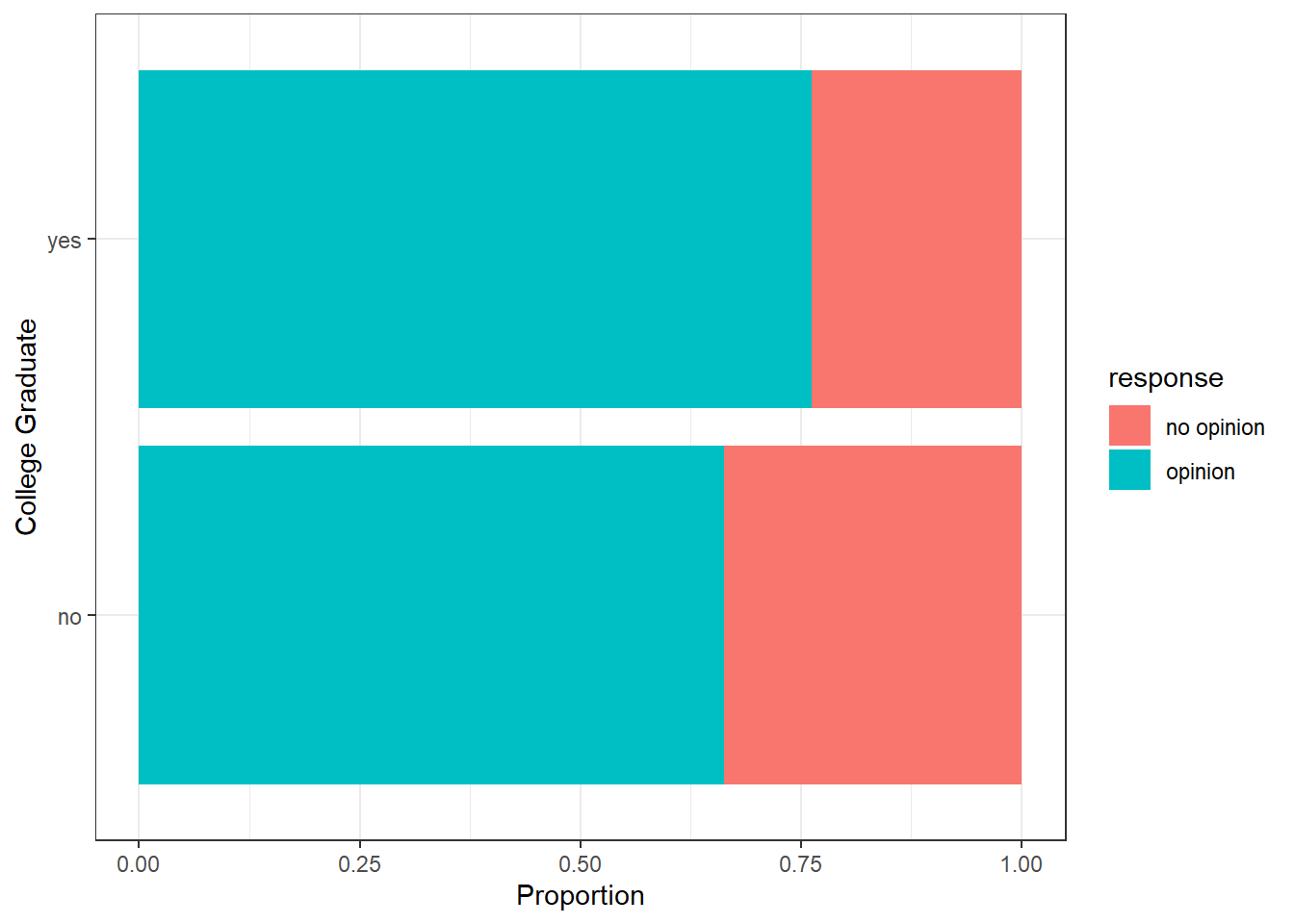
Calculate proportions
We will use the following code to show the proportions across the
rows which will tell us the proportions of each level of the
college_grad variable:
CC19
## Important: this code chunk uses the 'counts' data object created in CC17! Be sure to include that code chunk in any derivative worksheets.

# margin = 1 gives the row proportions.
# margin = 2 would give the column proportions
# using round (() ,3) to round to 3 digits.
row_proportions <- round(prop.table(counts, margin = 1), 2)

# Display the table of row proportions
row_proportions
##
## no opinion opinion
## no 0.34 0.66
## yes 0.24 0.76This seems to indicate that a larger proportion ( 72%) of respondents with a college degree indicated they had an opinion on drilling offshore in California. The proportion for those without a college degree that have an opinion on offshore drilling is 68%.
But is there sufficient evidence that whether or not the respondents had a college degree made a difference in whether or not they had an opinion on offshore drilling for oil?
State the Null and Alternative hypotheses
Null hypothesis: The proportions of Californian voters having an opinion on offshore drilling for voters who are a college graduate and for voters who are not a college graduate are equal.
Alternative hypothesis: The proportions of Californian voters having an opinion on offshore drilling for voters who are a college graduate and for voters who are not a college graduate are not equal.
Question: What is the direction of this hypothesis test?
Your answer:
State the Significance Level
Let’s set the significance level at 5% ( i.e., 0.05) here because nothing too serious will happen if we are wrong.
Testing the hypothesis
Step 1: Calculate the observed statistic
Calculate the observed statistic and store the results in a new data
object called delta.
CC20
delta_obs<- offshore %>%
  specify(response ~ college_grad, success = "opinion") %>%
  calculate(stat = "diff in props", order = c("yes", "no"))

# Display the observed difference
delta_obs
## Response: response (factor)
## Explanatory: college_grad (factor)
## # A tibble: 1 × 1
## stat
## <dbl>
## 1 0.0993Approximately 4% more college graduates have an opinion on offshore drilling than non-college graduates.
Step 2: Generate the Null Distribution
Generate the null distribution of the proportion of respondents with an opinion.
CC21
set.seed(123) #to insure consistent results

null_dist <- offshore %>%
  specify(response ~ college_grad, success = "opinion") %>%
  hypothesize(null = "independence") %>%
  generate(reps = 1000) %>%
  calculate(stat = "diff in props", order = c("yes", "no"))

null_dist  #display the data object
## Response: response (factor)
## Explanatory: college_grad (factor)
## Null Hypothesi...
## # A tibble: 1,000 × 2
## replicate stat
## <int> <dbl>
## 1 1 -0.00747
## 2 2 0.00224
## 3 3 0.0265
## 4 4 -0.00261
## 5 5 -0.0269
## 6 6 0.0411
## 7 7 0.00710
## 8 8 -0.0414
## 9 9 0.0362
## 10 10 0.0119
## # ℹ 990 more rowsNote we use the hypothesize function to set our null
hypothesis to be that of “independence”. If the two variables
response and `college_grad` are independent of each other,
i.e. there is no relationship between the two variables, we should see
no difference in the proportions of respondents with no opinion on
offshore drilling.
Step 3: Visualize the Null and the Observed Statistic
We need to calculate the means of each of the “reps” in the
null_dist data object.
CC22
visualize(null_dist) +
  shade_p_value(obs_stat = delta_obs, direction = "two-sided") +
   labs(x = "Difference in Proportion", y = "Count",
       title = "Null distribution of Difference in Proportions",
       subtitle = "Actual difference observed in the data is marked in red") +
  theme_bw()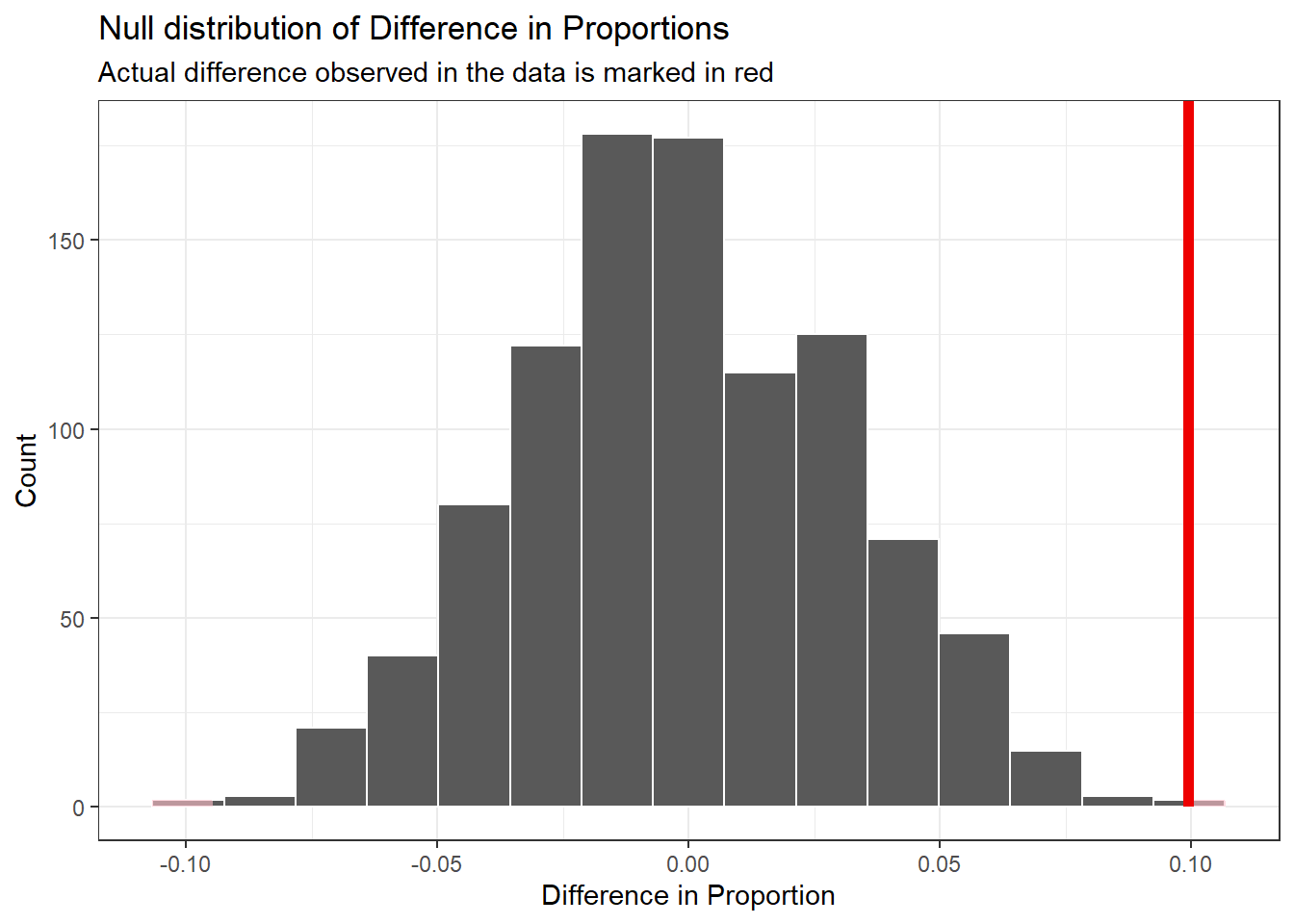
Step 4: Calculate the p-value
Calculate the p-value (“area” under the curve beyond
delta_obs in both directions) from the Null distribution
and the observed statistic delta_obs.
CC23
p_value <- null_dist %>%
  get_pvalue(obs_stat = delta_obs, direction = "both")

p_value  #print p_value
## # A tibble: 1 × 1
## p_value
## <dbl>
## 1 0.002Step 5: Decide if delta_obs is statistically significant
Compare the p-value with the significance level alpha. If the p-value is less than alpha, the Null hypothesis must be rejected.
CC24
# When reusing this code chunk, no changes are needed.

alpha <- 0.05

if(p_value <= alpha){
  print("Reject the Null Hypothesis")
} else {
    print("Fail to reject the Null Hypothesis")
}
## [1] "Reject the Null Hypothesis"Results and Conclusions
Because the p-value of approximately 0.002 is less than the significance level of 0.05, we reject the Null hypothesis of no difference.
We conclude that there is a significance difference in the proportions of California voters with an opinion on offshore drilling between those with a college degree and those without a college degree.
Or, said another way, whether or not a California voter has an opinion on offshore drilling is dependent upon whether or not they have a college degree.
Calculate confidence interval
The following code chunk will allow us to calculate a 95% confidence interval for the difference in the two proportions.
CC25
set.seed(123) #assure reproducibility

ci <- offshore %>%
  specify(response ~ college_grad, success = "opinion" ) %>%
  generate(reps = 1000, type="bootstrap") %>%
  calculate(stat = "diff in props", order = c("yes", "no")) %>%
  get_confidence_interval(level = 0.95)

#print the CI upper and lower limits
ci
## # A tibble: 1 × 2
## lower_ci upper_ci
## <dbl> <dbl>
## 1 0.0387 0.168The Null value of 0 difference is not contained in the CI . This
supports the conclusion that there is a significant difference in the
proportion having an opinion on offshore drilling between California
voters with and without a college degree.
Traditional hypothesis test
Complete all the above tasks with a traditional test for difference in two proportions. Note that all the above steps can be done with one line of code if a slew of assumptions are checked and verified. See Assumptions for Traditional Tests
The test is comparing the proportions of the response
variable for each level of the college_grad variable.
CC26
prop.test(table(offshore$college_grad, offshore$response), correct=FALSE)##
## 2-sample test for equality of proportions without continuity correction
##
## data: table(offshore$college_grad, offshore$response)
## X-squared = 9.9907, df = 1, p-value = 0.001573
## alternative hypothesis: two.sided
## 95 percent confidence interval:
## 0.03772522 0.16091078
## sample estimates:
## prop 1 prop 2
## 0.3367609 0.2374429This traditional two-proportions test has essentially the same results as we got with the Downey-Infer method. The p-value is approximately 0.0016 and the Null value of 0 difference is not found in the confidence interval. Again, the conclusion is that there is a significant difference in the proportions of the responses of college grads and non-college grades on off shore drilling.
Lab Assignment Submission
Important
When you are ready to create your final lab report, save the Lab-7-Rehearse1-Worksheet.Rmd lab file and then Knit it to PDF or Word to make a reproducible file.
Note that if you have difficulty getting the documents to Knit to either Word or PDF, and you cannot fix it, just save the completed worksheet and submit your .Rmd file for partial credit.
Submit your file in the M7.2 Lab 7 Rehearse(s): Hypothesis Tests Part 2-Proportions assignment area.
The Lab 7 Hypothesis Tests Part 2 Grading Rubric will be used.

Congrats! You have finished Rehearse 1 of Lab 7. Now go to Rehearse 2!


This
work was created by Dawn Wright and is licensed under a
Creative
Commons Attribution-ShareAlike 4.0 International License.
Date 4/18/26
Last Compiled 2026-04-18