Describing Data

Attribution: This lab is adapted and expanded from: Answering questions with data: Lab Manual, Matthew J. C. Crump, Anjali Krishnan, Stephen Volz, and Alla Chavarga 2019.

Describing comic sensibility is near impossible. It’s sort of an abstract silliness, that sometimes the joke isn’t the star.

–Dana Carvey

The purpose of this tutorial is to show you how to compute basic descriptive statistics, including measures of central tendency (mean, mode, median) and variation (range, variance, standard deviation).

General Goals

Practice using R code chunks
Compute measures of central tendency using software
Compute measures of variation using software
Ask some questions of a data set using descriptive statistics

Let’s get going in Posit Cloud!

Link to Posit Cloud

Log into your Posit Cloud account
Open the Lab 2 Exploring Data project.
Open the Lab2-Rehearse2-Describing-Data-Worksheet.Rmd file.

Important

Be sure to edit in your name and put in the current date in the proper locations at the top of the Lab2-Rehearse2-Describing-Data-Worksheet.

Also Important:

The free version of the Posit Cloud account is limited to 25 hours of operation per month. This should be plenty of time since each lab should take no more than 2 to 4 hours of work time. Normally, Posit Cloud will go into “sleep” mode when you have your account open but are not being active, but your clock keeps running for a bit each time.

We recommend you log out of your account when you take breaks, or pause for lunch/dinner. It only takes a few seconds to log back in.

And if you want to further explore Posit Cloud/RStudio beyond our class work, we recommend you install RStudio desktop as it has no time limit of hours used per month.

Packages

These two packages are needed for this portion of the lab. Be sure to run this code now and to load the packages when the instructions indicate. Note that the gapminder package will create several data objects which will show in your Environment.

Also understand you may get a warning that a package(s) are already installed. You can follow that instruction and let R restart.

hint Remember!

Remember to click on the green Copy icon in the upper left corner of the code chunk in this webpage and then use right-click Paste to put the code in the chunk area in the worksheet.

When you click on the small green Run triangle in the upper right corner of the r code chunk in the worksheet, it will run the code.

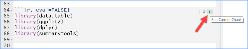
Note this example image above has four packages; we only need two for this Rehearse session.

Remember “Copy/Paste/Run”

CC1

library(tidyverse)
library(gapminder)

Descriptive Statistics Basics in R

We learned from the textbook that data we want to use ask and answer questions often comes with loads of numbers. Too many numbers to look at all at once. That’s one reason we use descriptive statistics. To reduce the big set of numbers to one or two summary numbers that tell us something about all of the numbers. R can produce descriptive statistics for you in many ways. There are base functions for most of the ones that you want. We’ll go over some R basics for descriptive statistics, and then use our these basic skills to ask some questions about real data.

1 Making numbers in R

1.1 Combine

In order to do descriptive statistics we need to put some numbers in a variable. You can also do this using the c() command, which stands for “combine”.

CC2

Remember to copy, paste and run the code chunk whenever you see the green copy icon in a code chunk.

my_numbers <- c(1,2,3,4)

We used the combine function to assign the four numbers to a variable named my_numbers with the <- symbol. You should see a my_numbers variable in your Environment tab/ Values section in the upper right window.

There are a few other handy ways to make numbers.

1.2 Sequence

We can use seq() to make a sequence. Here’s making the numbers from 1 to 100.

CC3

one_to_one_hundred <- seq(1,100,1)

The “syntax” - fancy word for the info we need to give the function - is seq(from 1 to 100, by 1’s).

hint Hint

If you want to get more information about a function, go to the Help tab in the Files window and search for the function name, “seq” in this case.

1.3 Repeat

We can repeat things, using rep. Here’s making 10 5s, and 25 1s using the rep function. Then we combine the two to create a variable we name “all_together_now.” In R, we call a variable like this a numeric”vector. You should see it in the “Values” section of the Environment window: num [1:35] 5555….

Don’t worry too much about the term “vector.” It just means we have a variable in the Environment which is a collection of all 35 numbers we have created with the rep functions.

CC4

rep(5,10)

 [1] 5 5 5 5 5 5 5 5 5 5

rep(1,25)

 [1] 1 1 1 1 1 1 1 1 1 1 1 1 1 1 1 1 1 1 1 1 1 1 1 1 1

all_together_now <- c(rep(5,10),rep(1,25))

1.4 Sum

Let’s play with the number 1 to 100. First we create a new variable and give it the sequence of numbers 1 to 100 with the seq function.

Then, let’s use the sum() function to add them up: 1+2+3+4+…99+100. You can Google this and find the sum to be 5050.

CC5

one_to_one_hundred <- seq(1,100,1)
sum(one_to_one_hundred)

[1] 5050

1.5 Length

We put 100 numbers into the variable one_to_one_hundred, so we know how many numbers there are in there. How can we get R to tell us the number of numbers/values in a variable we are unsure of? We use length() for that.

CC6

length(one_to_one_hundred)

[1] 100

2 Central Tendency

Often we would like to have just one number we can use to represent our data. A reasonable value we can use would be one that is in the center of our data.

2.1 Mean

Remember the mean of some numbers is their sum, divided by the number of numbers. We can compute the mean like this:

CC7

sum(one_to_one_hundred)/length(one_to_one_hundred)

Or, we could just use the mean() function like this:

CC8

mean(one_to_one_hundred)

2.2 Median

The median is the number in the exact middle of the numbers ordered from smallest to largest. If there are an even number of numbers (no number in the middle), then we take the number in between the two (decimal .5). Use the median function. There are only 3 numbers in the code chunk below. The middle one is 2, that should be the median.

CC9

median(c(1,2,3))

Try it: add 4 to the code chunk above to give 4 numbers, i.e. 1,2,3,4, and run the code again.

Reflect 1

What is the median now? Your answer here:

Now let’s see what having a large number does to the median. Replace the 4 with 100:

CC10

median(c(1,2,3,100))

Reflect 2

Did the median change with the large 4th number? Your answer here:

2.3 Mode

R does not have a base function for the Mode. You would have to write one for yourself. Here is an example of writing your own mode function, and then using it.

Note I searched how to do this on Google, and am using the mode defined by this answer on stack overflow

Remember, the mode is the most frequently occurring number in the set. Below 1 occurs the most in this set, so the mode will be one.

CC11

my_mode <- function(x) {
  ux <- unique(x)
  ux[which.max(tabulate(match(x, ux)))]
}

my_mode(c(1,1,1,1,1,1,1,2,3,4))

[1] 1

3 Variation

We often want to know how variable the numbers are. We are going to look at descriptive statistics to describe this such as the range, variance, the standard deviation, and a few others.

First, let’s remind ourselves what variation looks like (it’s when the numbers are different). We will sample 100 numbers from a normal distribution (don’t worry about this yet - we will discuss distributions in the next lab), with a mean of 10, and a standard deviation of 5, and then make a histogram so we can see the variation around 10.

CC12

sample_numbers <- rnorm(100,10,5)
hist(sample_numbers)

Reflect 3

Think about this: run the above code chunk several more times and observe the histogram. What do you think is happening?

Write your answer here:

Another word for “variation” is “distribution.” A histogram is a good tool for visualizing the distribution of a numeric variable. Check out this page for more info on histograms: https://www.data-to-viz.com/graph/histogram.html

3.1 Range

The range is the minimum and maximum values in the set, we use the range function.

CC13

# the range function finds the min and the max values in a set of numbers
x <- range(sample_numbers)
# the round function rounds values to a specified number of decimal places
round(x, digits = 2)

Note: because we used a random sample using the above code chunk to create sample_numbers, your values for range and the following statistics will likely be different from what is in these instructions or what another student might get.

3.2 Variance

While the range is useful, it uses just two values in the data set. We can use the variance to inform us more about the variation in all the data points. We can find the sample variance using var.

Note, the formula for Variance divides by (n-1), the number of observations minus 1 because this is a sample and not the entire population.

CC14

var(sample_numbers)

3.3 Standard Deviation

sd = standard deviation

We can find the sample standard deviation using the sd function. Note, it also divides by (n-1) because this is a sample and not the entire population.

CC15

sd(sample_numbers)

3.3.1

The standard deviation is just the square root of the variance as we see here:

CC16

sqrt(var(sample_numbers))

4 All Descriptives

Let’s put all of the descriptives and other functions so far in one place:

CC17

sample_numbers <- rnorm(100,10,5)

sum(sample_numbers)
length(sample_numbers)
mean(sample_numbers)
median(sample_numbers)
my_mode(sample_numbers)
range(sample_numbers)
var(sample_numbers)
sd(sample_numbers)

4.1 Descriptives by conditions

Sometimes you will have a single variable with some numbers, and you can use the above functions to find the descriptives for that variable. Other times (most often in this course), you will have a big data frame of numbers, with different numbers in different conditions. You will want to find descriptive statistics for each of the sets of numbers inside each of the conditions. Fortunately, this is where R really shines, it does it all for you in one go.

Let’s illustrate the problem. Here we make a data frame with 10 numbers in each condition. There are 10 conditions, each labelled, A, B, C, D, E, F, G, H, I, J.

CC18

scores <- rnorm(100,10,5)
conditions <- rep(c("A","B","C","D","E","F","G","H","I","J"), each =10)
my_df <- data.frame(conditions,scores)

If you look at the my_df data frame in the Environment window, you will see it has 100 rows. There are 10 rows for each condition with a label in the conditions column, and 10 scores for each condition in the scores column.

hint Hint

Another name for “condition” is “variable” or “values”, the latter is what R uses in the Environment window.

4.2 Means of each condition

What if you wanted to know the mean of the scores in each condition? You would want to find 10 means.

4.2.1 The slow way to do it would be like this:

CC19

mean(my_df[my_df$conditions=="A",]$scores)
mean(my_df[my_df$conditions=="B",]$scores)
mean(my_df[my_df$conditions=="C",]$scores)
# and then keep going

Nobody wants to do that! Not, me I stopped doing it that way. You should too.

4.2.2 group_by and summarise

We can easily do everything all at once using the group_by and summarise function from the dplyr package. Just watch:

CC20

library(dplyr)

my_df %>%
  group_by(conditions) %>%
  summarise(means = mean(scores))

A couple of things now. First, you may notice R uses the word “tibble” for the new data frame, e.g.”# A tibble: 10 x 2.” You don’t have to remember what a tibble is, but it just is a way to make the data print out a little nicer in the view in your Editor window. But the printout when you Knit may not be as nice as a tibble.

4.2.3 Make it look nice

Let’s fix that. We put the results of our code into a new variable, then we use knitr::kable to print it out nicely when we knit the document:

CC21

summary_df <- my_df %>%
               group_by(conditions) %>%
               summarise(means = mean(scores))

knitr::kable(summary_df)

Hint

If you want to know more about how to change the format of the table, e.g. the number of decimal places, etc. , check out the web page Formatting Tables in R

4.3 Multiple descriptives

The best thing about the dplyr method, is that we can add more than one function, and we’ll get more than one summary returned, all in a nice format. Let’s add the standard deviation:

CC22

summary_df <- my_df %>%
               group_by(conditions) %>%
               summarise(means = mean(scores),
                         sds = sd(scores))

knitr::kable(summary_df)

4.3.1 Min and Max

We’ll add the min and the max too:

CC23

summary_df <- my_df %>%
               group_by(conditions) %>%
               summarise(means = mean(scores),
                         sds = sd(scores),
                         min = min(scores),
                         max = max(scores))

knitr::kable(summary_df)

5 Describing gapminder

Now that we know how to get descriptive statistics from R, we can do this will some real data. Let’s quickly get some basic statistics about the gapminder data.

CC24

library(gapminder)
library(tidyverse)
gapminder_df <- gapminder

Note: The above code will only work if you have installed the gapminder package. Make sure you are connected to the Internet. Then choose the Packages tab from the bottom right panel, and choose install. Then search for gapminder, choose it, and install it.

5.1 Life Expectancy

What are some descriptive statistics for Life expectancy by continent?

Copy the code from the last part of “descriptives” above, i.e., code chunk 23. We have done this part for you in the code block below.

Then:

Change the source data frame in the first line from “my_df” to “gapminder_df”.
Change the group by variable from “conditions” to “continent”.
Change the summarize variable names from “scores” to “lifeExp”.

CC25

summary_df <- my_df  %>%
               group_by(conditions) %>%
               summarize(means = mean(scores),
                         sds = sd(scores),
                         min = min(scores),
                         max = max(scores))

knitr::kable(summary_df)

Lab Assignment Submission

Important

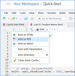
When you are ready to create your final lab report, save the Lab-02-Rehearse2-Describing-Data-Worksheet.Rmd file and then Knit it to PDF or Word to make a reproducible file. This image below shows you how to select the knit document file type.

Note if you encounter difficulty getting your worksheet to Knit, you may submit your Lab2-Rehearse2-Describing-Data-Worksheet.Rmd file saved with your work instead.

Ask your instructor to help you sort out the issues if you have time.

Submit your file in the Canvas M2.4 Lab 2 Rehearse(s): Exploring Data Canvas assignment area.

The Lab 2 Exploring Data Grading Rubric will be used.