About the unvotes package
Dawn Wright
9/1/2022
unvotes package
Citation: Erik Voeten “Data and Analyses of Voting in the UN General Assembly” Routledge Handbook of International Organization, edited by Bob Reinalda (published May 27, 2013)
The unvotes package contains three datasets, each set up as a data frame which is also called a data table. First is the history of each country’s vote. These are represented in the un_votes dataset, with one row for each country/vote pair:
Note that packages( also called “libraries”) must be installed before they are loaded. Usually, RStudio will notify you to install the packages required in a file. We use the library() function to load the libraries after they have been installed. This code below just “loads” the two packages, dplyr and unvotes.
library(dplyr)
library(unvotes)
#use the name of the data set to print out a "tibble" or the first 10 rows of the data set.
un_votes
## # A tibble: 869,937 × 4
## rcid country country_code vote
## <dbl> <chr> <chr> <fct>
## 1 3 United States US yes
## 2 3 Canada CA no
## 3 3 Cuba CU yes
## 4 3 Haiti HT yes
## 5 3 Dominican Republic DO yes
## 6 3 Mexico MX yes
## 7 3 Guatemala GT yes
## 8 3 Honduras HN yes
## 9 3 El Salvador SV yes
## 10 3 Nicaragua NI yes
## # … with 869,927 more rows
## # ℹ Use `print(n = ...)` to see more rows“rcid” stands for roll call id, the number of the roll call vote starting back when the UN was established in 1946. The other columns are self-explanatory with the variable “vote” being yes if the country voted “yes” on that roll call vote.
The unvotes package also contains a second dataset of information about each roll call vote, including the UN Session number and date, the description of the roll call vote, and relevant resolution that was voted on:
un_roll_calls## # A tibble: 6,202 × 9
## rcid session importantvote date unres amend para short descr
## <int> <dbl> <int> <date> <chr> <int> <int> <chr> <chr>
## 1 3 1 0 1946-01-01 R/1/66 1 0 AMENDMENTS,… "TO …
## 2 4 1 0 1946-01-02 R/1/79 0 0 SECURITY CO… "TO …
## 3 5 1 0 1946-01-04 R/1/98 0 0 VOTING PROC… "TO …
## 4 6 1 0 1946-01-04 R/1/107 0 0 DECLARATION… "TO …
## 5 7 1 0 1946-01-02 R/1/295 1 0 GENERAL ASS… "TO …
## 6 8 1 0 1946-01-05 R/1/297 1 0 ECOSOC POWE… "TO …
## 7 9 1 0 1946-02-05 R/1/329 0 0 POST-WAR RE… "TO …
## 8 10 1 0 1946-02-05 R/1/361 1 1 U.N. MEMBER… "TO …
## 9 11 1 0 1946-02-05 R/1/376 0 0 TRUSTEESHIP… "TO …
## 10 12 1 0 1946-02-06 R/1/394 1 1 COUNCIL MEM… "TO …
## # … with 6,192 more rows
## # ℹ Use `print(n = ...)` to see more rowsFrom inspecting the tibble for this data set we can see there have been over 6200 roll call votes since the beginning of the UN in 1946.
The 3rd data set contains data on just six selected issues for which the UN has had numerous roll call votes. Note that there are many more issues not included in this data “subset” of UN votes.
un_roll_call_issues## # A tibble: 5,745 × 3
## rcid short_name issue
## <int> <chr> <fct>
## 1 77 me Palestinian conflict
## 2 9001 me Palestinian conflict
## 3 9002 me Palestinian conflict
## 4 9003 me Palestinian conflict
## 5 9004 me Palestinian conflict
## 6 9005 me Palestinian conflict
## 7 9006 me Palestinian conflict
## 8 128 me Palestinian conflict
## 9 129 me Palestinian conflict
## 10 130 me Palestinian conflict
## # … with 5,735 more rows
## # ℹ Use `print(n = ...)` to see more rowsBefore we merge the three data sets, let’s take a look at how many roll call votes there have been on these six issues.
library(dplyr)
count(un_roll_call_issues, issue, sort = TRUE)
## # A tibble: 6 × 2
## issue n
## <fct> <int>
## 1 Arms control and disarmament 1092
## 2 Palestinian conflict 1061
## 3 Human rights 1015
## 4 Colonialism 957
## 5 Nuclear weapons and nuclear material 855
## 6 Economic development 765Explanation of the code chunk used:
We use the count function in the dplyr library to first sort the six issues into groups and then count the number of votes on each group. A function in R has the form of function_name( ). In the parentheses, we first list the name of the dataset un_roll_call_issues, the variable of interest [issue], and indicate we do want to sort [sort = TRUE].
We can perform more analyses if we put the data in the three data sets into one data table. We can do this by merging or joining the three using a common variable, rcid.
library(dplyr)
unvotes1 <- un_votes %>%
  inner_join(un_roll_calls, by = "rcid") %>%
  inner_join(un_roll_call_issues, by = "rcid")
#this prints a tibble of unvotes
unvotes1
## # A tibble: 857,878 × 14
## rcid country count…¹ vote session impor…² date unres amend para
## <dbl> <chr> <chr> <fct> <dbl> <int> <date> <chr> <int> <int>
## 1 6 United Stat… US no 1 0 1946-01-04 R/1/… 0 0
## 2 6 Canada CA no 1 0 1946-01-04 R/1/… 0 0
## 3 6 Cuba CU yes 1 0 1946-01-04 R/1/… 0 0
## 4 6 Dominican R… DO abst… 1 0 1946-01-04 R/1/… 0 0
## 5 6 Mexico MX yes 1 0 1946-01-04 R/1/… 0 0
## 6 6 Guatemala GT no 1 0 1946-01-04 R/1/… 0 0
## 7 6 Honduras HN yes 1 0 1946-01-04 R/1/… 0 0
## 8 6 El Salvador SV abst… 1 0 1946-01-04 R/1/… 0 0
## 9 6 Nicaragua NI yes 1 0 1946-01-04 R/1/… 0 0
## 10 6 Panama PA abst… 1 0 1946-01-04 R/1/… 0 0
## # … with 857,868 more rows, 4 more variables: short <chr>, descr <chr>,
## # short_name <chr>, issue <fct>, and abbreviated variable names
## # ¹country_code, ²importantvote
## # ℹ Use `print(n = ...)` to see more rows, and `colnames()` to see all variable names#this prints out all the column/variable names in the unvotes1 data set
colnames(unvotes1)## [1] "rcid" "country" "country_code" "vote"
## [5] "session" "importantvote" "date" "unres"
## [9] "amend" "para" "short" "descr"
## [13] "short_name" "issue"This code chunk begins by creating a new dataframe named “unvotes1” using the assign characters <- to put the data in the original un_votes data set into “unvotes1.”
The next symbol is call the pipe operator because it “pipes” or transfers the result of the assignment to begin the joining process. You can think of the pipe operator %>% as saying “and then.”
For example, assign the data in un_votes to the new data set unvotes1 “and then” join that data set with the data in un_roll_calls using the common variable “rcid” to match up the rows.
Finally, we have another pipe operator so “and then” use the inner_join function to merge the data in the last data set into unvotes1.
One could then count how often each country votes “yes” on a resolution in each year:
library(lubridate)

by_country_year <- unvotes1 %>%
  group_by(year = year(date), country) %>%
  summarize(votes = n(),
            percent_yes = mean(vote == "yes"))

by_country_year
## # A tibble: 10,452 × 4
## # Groups: year [73]
## year country votes percent_yes
## <dbl> <chr> <int> <dbl>
## 1 1946 Afghanistan 12 0.25
## 2 1946 Argentina 27 0.778
## 3 1946 Australia 27 0.556
## 4 1946 Belarus 27 0.370
## 5 1946 Belgium 27 0.630
## 6 1946 Bolivia 27 0.741
## 7 1946 Brazil 27 0.704
## 8 1946 Canada 26 0.808
## 9 1946 Chile 27 0.741
## 10 1946 Colombia 25 0.28
## # … with 10,442 more rows
## # ℹ Use `print(n = ...)` to see more rowsAfter which this can be visualized for one or more countries:
library(ggplot2)
theme_set(theme_bw())

#This next line creates a new data object "countries" consisting of just the names of the four listed countries.

countries <- c("United States", "United Kingdom", "India", "France")

#Next we begin with the "by_country_year" data set
# and then
# Filter out all but the four countries in the "countries" data object
# and then begin our plot using the ggplot function
by_country_year %>%
  filter(country %in% countries) %>%
  ggplot(aes(year, percent_yes, color = country)) +
  geom_line() +
  ylab("% of votes that are 'Yes'")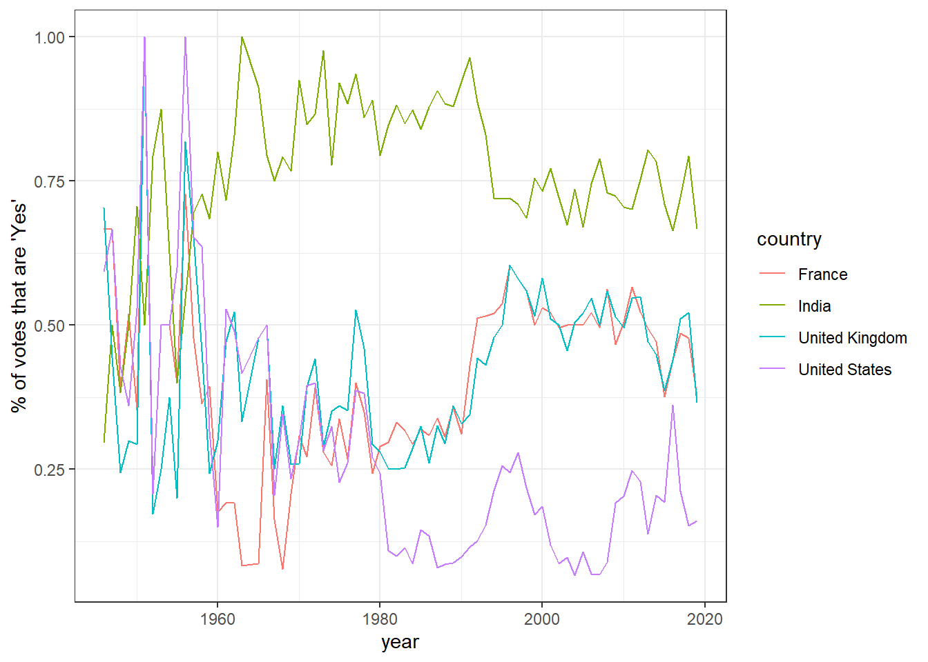
Look at how the voting record of the US has changed on each of the six issues:
unvotes1 %>%
  filter(country == "United States") %>%
  group_by(year = year(date), issue) %>%
  summarize(votes = n(),
            percent_yes = mean(vote == "yes")) %>%
  filter(votes > 5) %>%
  ggplot(aes(year, percent_yes)) +
  geom_point() +
  geom_smooth(se = FALSE) +
  facet_wrap(~ issue)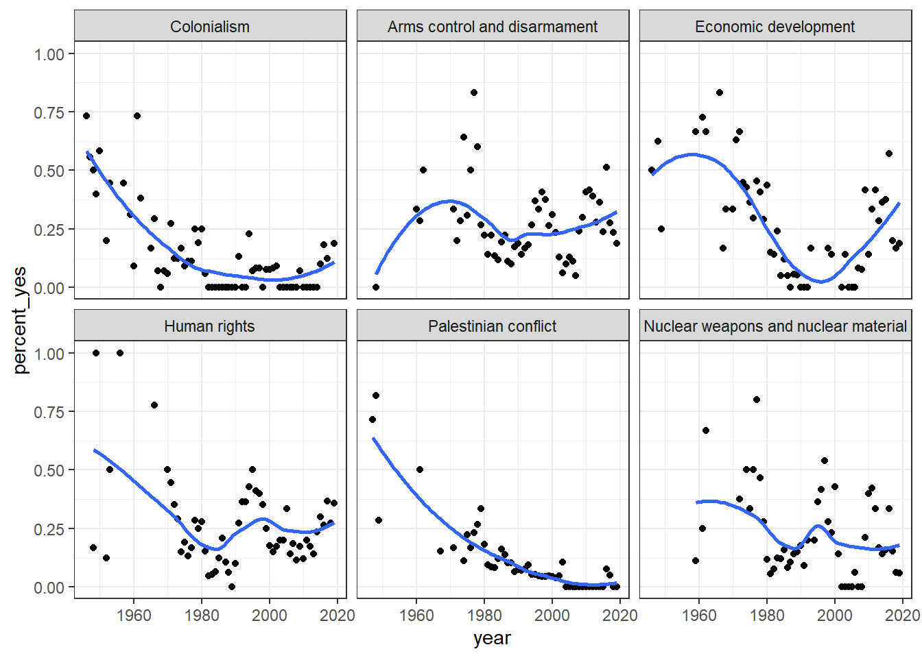
Return to the debrief[https://bus-data-lit-lab.netlify.app/debrief.html]