Attribution: This lab is an adaptation of a case study How much is a Fireplace Worth? by Dick De Veaux Link to De Veaux Case Study

1 Lab 4 Rehearse 2 Regression

1.1 Posit Cloud

Log into your Posit Cloud account. Link to Posit Cloud
Open the Lab 4 Relationships project.
Open the Lab-04-Rehearse2-Worksheet.Rmd.

**IMPORTANT!

Remember to rename this file to include your name in place of “Student-Name” at the top of the page.

Other than entering your name to replace Student Name and changing the date to the current date, do not change anything in the head space.

2 Load Packages

Let’s load the packages we will need for this rehearse. Remember we may get some messages and warnings. They are generally nothing to worry about, but you should learn to scan them as you get more experience with R.

CC3

library(ggpubr)
library(tidyverse)
library(broom)

3 Regression Models

In the first Rehearse in lab 4, we discussed correlation, created scatter plots showing a possible relationship, calculated a correlation coefficient, and added a trend line. That trend line is also called a regression line of best fit. We can calculate the equation for a trend line and use that equation to predict the values of the response variable - usually the variable plotted on the y-axis - given a value for the independent or predictor x variable.

But we will find, like with spurious correlations, that a single predictor variable may not give us the whole story. There are usually other variables at play in determining a response variable’s value. We will explore this fact in this Rehearse.

3.1 Zillow

The website Zillow estimates the home prices for over 100,000,000 homes around the United States. (Well, actually they call them Zestimates.) In their own words,“We use proprietary automated valuation models that apply advanced algorithms to analyze our data to identify relationships within a specific geographic area, between this home-related data and actual sales prices. Home characteristics, such as square footage, location or the number of bathrooms, are given different weights according to their influence on home sale prices in each specific geography over a specific period of time, resulting in a set of valuation rules, or models that are applied to generate each home’s Zestimate. Specifically, some of the data we use in this algorithm include:

Physical attributes: Location, lot size, square footage, number of bedrooms and bathrooms and many other details.
Tax assessments: Property tax information, actual property taxes paid, exceptions to tax assessments and other information provided in the tax assessors’ records.
Prior and current transactions: Actual sale prices over time of the home itself and comparable recent sales of nearby homes

Currently, we have data on 110 million homes and Zestimates and Rent Zestimates on approximately 100 million U.S. homes. (Source: Zillow Internal, March 2013) ” ———–

3.2 About this Rehearse

Everyone’s heard the real estate adage that the three most important things in real estate are: location, location and location. And notice that it’s first on Zillow’s list of variables. We’re not going to try to compete with Zillow here. Instead, we’ll make things simpler by keeping the location restricted to Saratoga County, New York. We’ll explore some data on home prices to see if we can come up with our own model. In particular, we’ll study how much more a house can fetch if it has a fireplace in it. We’ll use the prices of 1000 homes collected from public records about 8 years ago in Saratoga County, New York by a student studying at Williams College.

Some of our goals for this study include building and reinforcing skills for

Examining the Distribution of a Variable
Comparing two groups via boxplots and summary statistics
Summarizing the relationship between variables using linear regression
- We first use simple regression.
- Then we add an indicator variable (dummy variable) to adjust the intercept for two groups.
- Finally, we introduce an interaction term to adjust the slopes for the two groups.
The result is a multiple regression model using interaction terms to create a more complex and realistic model.

4 Exploration

We start by exploring all the variables. Of course, we first need to bring in the data. We import the data from a website using the simple command read.delim(“http://sites.williams.edu/rdeveaux/files/2014/09/Saratoga.txt”).

We can then look at a summary – and we notice that some of the categorical variables (Fuel Type, Waterfront etc) are treated as numerical.

CC4

# read in data from the web 
real=read.delim("http://sites.williams.edu/rdeveaux/files/2014/09/Saratoga.txt")  

options(width=100)
summary(real)

     Price           Lot.Size         Waterfront            Age           Land.Value    
 Min.   :  5000   Min.   : 0.0000   Min.   :0.000000   Min.   :  0.00   Min.   :   200  
 1st Qu.:145000   1st Qu.: 0.1700   1st Qu.:0.000000   1st Qu.: 13.00   1st Qu.: 15100  
 Median :189900   Median : 0.3700   Median :0.000000   Median : 19.00   Median : 25000  
 Mean   :211967   Mean   : 0.5002   Mean   :0.008681   Mean   : 27.92   Mean   : 34557  
 3rd Qu.:259000   3rd Qu.: 0.5400   3rd Qu.:0.000000   3rd Qu.: 34.00   3rd Qu.: 40200  
 Max.   :775000   Max.   :12.2000   Max.   :1.000000   Max.   :225.00   Max.   :412600  
 New.Construct      Central.Air       Fuel.Type       Heat.Type       Sewer.Type     Living.Area  
 Min.   :0.00000   Min.   :0.0000   Min.   :2.000   Min.   :2.000   Min.   :1.000   Min.   : 616  
 1st Qu.:0.00000   1st Qu.:0.0000   1st Qu.:2.000   1st Qu.:2.000   1st Qu.:2.000   1st Qu.:1300  
 Median :0.00000   Median :0.0000   Median :2.000   Median :2.000   Median :3.000   Median :1634  
 Mean   :0.04688   Mean   :0.3675   Mean   :2.432   Mean   :2.528   Mean   :2.695   Mean   :1755  
 3rd Qu.:0.00000   3rd Qu.:1.0000   3rd Qu.:3.000   3rd Qu.:3.000   3rd Qu.:3.000   3rd Qu.:2138  
 Max.   :1.00000   Max.   :1.0000   Max.   :4.000   Max.   :4.000   Max.   :3.000   Max.   :5228  
  Pct.College       Bedrooms       Fireplaces       Bathrooms       Rooms       
 Min.   :20.00   Min.   :1.000   Min.   :0.0000   Min.   :0.0   Min.   : 2.000  
 1st Qu.:52.00   1st Qu.:3.000   1st Qu.:0.0000   1st Qu.:1.5   1st Qu.: 5.000  
 Median :57.00   Median :3.000   Median :1.0000   Median :2.0   Median : 7.000  
 Mean   :55.57   Mean   :3.155   Mean   :0.6019   Mean   :1.9   Mean   : 7.042  
 3rd Qu.:64.00   3rd Qu.:4.000   3rd Qu.:1.0000   3rd Qu.:2.5   3rd Qu.: 8.250  
 Max.   :82.00   Max.   :7.000   Max.   :4.0000   Max.   :4.5   Max.   :12.000

So we need to do some data processing – telling the software that the numbers indicating Fuel Type (2-4), Heat Type (2-4), Waterfront (0 or 1) etc. are categorical. In R, categorical variables are called factors.

We can also give the categories labels inside the factor() function. By consulting with the Director of Data Processing of Saratoga County, De Veaux was able to assign the actual definitions of the numeric codes to the various levels.

De Veaux also created some new variables based on the original variables. The original variable Fireplace is the actual number of fireplace in the house. De Veaux created two variables from it: Fireplace is a 0/1 or Yes/No variable indicating presence of a fireplace and the new coding for Fireplaces uses just three levels: “None”,“1” and “2 or more”. Similarly, Beds is an ordered categorical variable created from Bedrooms.

Important

The code in the next chunk is complicated and is beyond the scope of our course. It is presented for completeness but you are not responsible for working with this particular code chunk. But this is part of “data wrangling” someone often has to do.

[This code chunk is already in your worksheet.]

CC5

real$Fuel.Type=factor(real$Fuel.Type,labels=c("Gas","Electric","Oil")) # Turn numbers into categories
real$Sewer.Type=factor(real$Sewer.Type,labels=c("None","Private","Public"))
real$Heat.Type=factor(real$Heat.Type,labels=c("Hot Air","Hot Water","Electric"))
real$Waterfront=factor(real$Waterfront,labels=c("No","Yes"))
real$Central.Air=factor(real$Central.Air,labels=c("No","Yes"))
real$New.Construct=factor(real$New.Construct,labels=c("No","Yes"))
real$Fireplace=factor(real$Fireplaces==0,labels=c("No","Yes"))
real$Fireplaces=factor(real$Fireplaces)
real$Fireplace=factor(real$Fireplaces==0,labels=c("Yes","No"))
levels(real$Fireplaces)=c("None","1","2 or more","2 or more","2 or more")
real$Beds=as.factor(real$Bedrooms)
levels(real$Beds)=c("2 or fewer","2 or fewer","3","4 or more","4 or more","4 or more","4 or more")

Running the summary again, we see that it looks much better:

Note: we included code to save the real data frame to our data folder too.

CC6

 # put a copy of the wrangled real into the workspace data folder
write.csv(real, "./data/real.csv")
 # show the new summary of real
summary(real)

     Price           Lot.Size       Waterfront      Age           Land.Value     New.Construct
 Min.   :  5000   Min.   : 0.0000   No :1713   Min.   :  0.00   Min.   :   200   No :1647     
 1st Qu.:145000   1st Qu.: 0.1700   Yes:  15   1st Qu.: 13.00   1st Qu.: 15100   Yes:  81     
 Median :189900   Median : 0.3700              Median : 19.00   Median : 25000                
 Mean   :211967   Mean   : 0.5002              Mean   : 27.92   Mean   : 34557                
 3rd Qu.:259000   3rd Qu.: 0.5400              3rd Qu.: 34.00   3rd Qu.: 40200                
 Max.   :775000   Max.   :12.2000              Max.   :225.00   Max.   :412600                
 Central.Air    Fuel.Type        Heat.Type      Sewer.Type    Living.Area    Pct.College   
 No :1093    Gas     :1197   Hot Air  :1121   None   :  12   Min.   : 616   Min.   :20.00  
 Yes: 635    Electric: 315   Hot Water: 302   Private: 503   1st Qu.:1300   1st Qu.:52.00  
             Oil     : 216   Electric : 305   Public :1213   Median :1634   Median :57.00  
                                                             Mean   :1755   Mean   :55.57  
                                                             3rd Qu.:2138   3rd Qu.:64.00  
                                                             Max.   :5228   Max.   :82.00  
    Bedrooms         Fireplaces    Bathrooms       Rooms        Fireplace         Beds    
 Min.   :1.000   None     :740   Min.   :0.0   Min.   : 2.000   Yes:988   2 or fewer:355  
 1st Qu.:3.000   1        :942   1st Qu.:1.5   1st Qu.: 5.000   No :740   3         :822  
 Median :3.000   2 or more: 46   Median :2.0   Median : 7.000             4 or more :551  
 Mean   :3.155                   Mean   :1.9   Mean   : 7.042                             
 3rd Qu.:4.000                   3rd Qu.:2.5   3rd Qu.: 8.250                             
 Max.   :7.000                   Max.   :4.5   Max.   :12.000

Reflection:

How many homes have more than 1 fireplace?

Your answer here:

4.1 Getting Started

A summary provides a good way to see how the variables are treated (as quantitative or categorical) and whether they are inundated with missing values.

However, don’t spend too much time examining variables this way – graphical displays, such as histograms and bar charts are a much better way to go.

Our response variable – the variable we’re trying to predict – is house price. Here’s a histogram.

CC7

options(scipen=1000)
with(real,hist(Price,col="#328da8",nclass=30,main="",xlab="Price ($)", ylab="Number of homes"))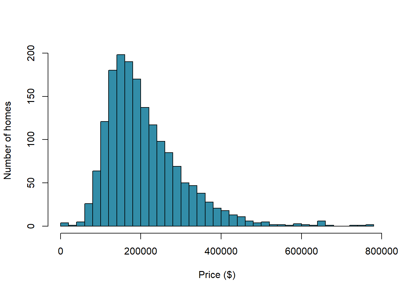

Depending upon how much room is available to show the plot, and how large or small the values are, you may see the values displayed in scientific notation. 2e+05 is equivalent to 2 multiplied by 10 to the +5 power or 200,000. 2e-05 would be equivalent to 2 multiplied by 10 to the -5 power or 0.00002.

However, we have used the “options(scipen=1000)” to prevent R from using scientific notation in the remainder of this document. See scipen

Reflection

How are house prices distributed? Would you consider them approximately Normally distributed? Why or Why not?

Your answer here:

4.2 House Size

Clearly, the size of the house is an important factor when considering the price. Here’s a histogram of the sizes (in square feet). How would you describe the distribution of house sizes?

CC8

with(real,hist(Living.Area,col="#FFA500",nclass=30,main="",xlab="Living Area (sq.ft)", ylab="Number of Homes"))

4.3 Fireplaces

Are houses with fireplaces generally more expensive than houses without? Let’s try a simple comparison of the prices for the two groups – those without and those with fireplaces. A box plot is a great way to display the differences. The dark line in the “middle” of the boxes represents the median or middle prices and you can definitely see a difference. We will calculate the difference in the mean prices next.

CC9

with(real,boxplot(Price~Fireplace,col=c("#FFA500","#328da8")))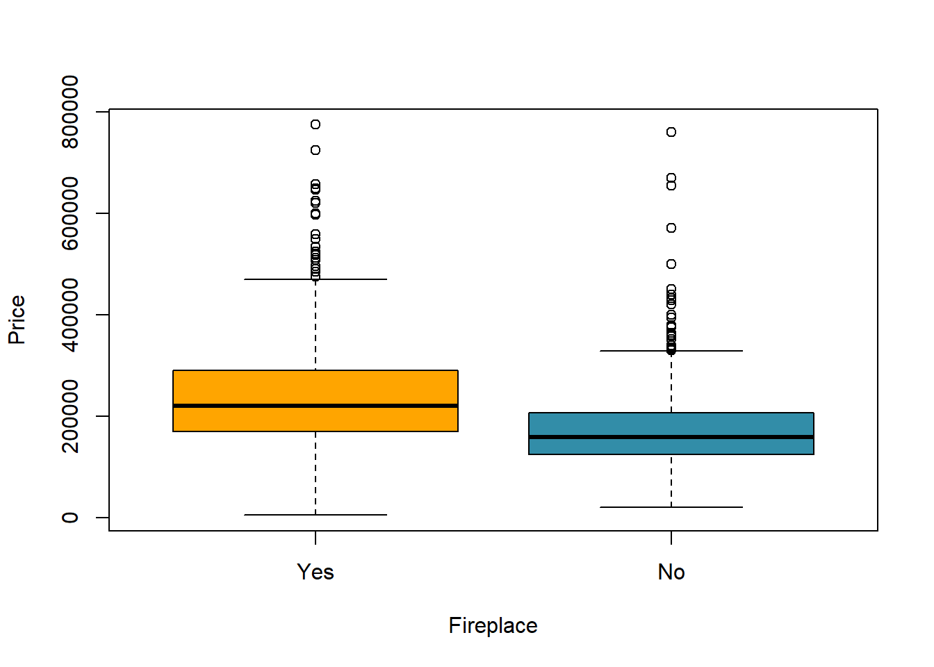

Reflection

The box plots and the histogram are telling us similar stories about the data. The dark lines in the boxes are the medians of the distributions, the “middles.” The small circles are unusual values - outliers. But having the two box plots side by side allows us to compare them.

Which group of homes has the higher median price?

Your answer here:

Let’s calculate some descriptive statistics using code chunk 25 from section 5.1 in the Lab 2 Rehearse 2 Describing Data:

CC10

summary_df <- real %>%
  #Fireplace variable has two levels: Yes and No
               group_by(Fireplace) %>%
               summarise(means = mean(Price),
               sds = sd(Price),
               min = min(Price),
               max = max(Price))

knitr::kable(summary_df)

Fireplace	means	sds	min	max
Yes	239914.0	102357.59	5000	775000
No	174653.4	78836.35	20000	760000

Let’s calculate the difference in average price between homes with and without fireplace.

CC11

fp_price <- real %>%
  filter(Fireplace %in% c("Yes")) %>%
  summarize(mean = mean(Price))
  
fp_price

So, the mean price of a home with a fireplace is $239,914.

CC12

no_fp_price <- real %>%
  filter(Fireplace %in% c("No")) %>%
  summarize(mean = mean(Price))
  
no_fp_price

And the mean price of homes without a fireplace is $174,653.

CC13

difference <- fp_price - no_fp_price
difference

The houses with fireplaces are more expensive. In fact, they are $65,261 more expensive, on average.

So, is a fireplace worth about $65,000 ? If you’re thinking of selling a house that doesn’t have a fireplace should you invest $50,000 to put one in?

4.4 What about other Variables?

Unless we have data from a designed experiment it is impossible to conclude that a change in one variable is the cause for the changes in another. Looking at differences in averages between groups is one of the most common ways to be led to make such false conclusions. While we can never assign cause, we can do better by adjusting for other variables that we know also contribute to the changes. This is the basic idea behind epidemiological, or case/control studies.

You may recall having read in a report “We controlled for variable x…”

From Minitab Blog,

“What does it mean to control for the variables in the model? It means that when you look at the effect of one variable in the model, you are holding constant all of the other predictors in the model. … You explain the effect that changes in one predictor (variable) have on the response (variable) without having to worry about the effects of the other predictors. In other words, you can isolate the role of one variable from all of the others in the model. And, you do this simply by including the variables in your model. It’s beautiful!

Running a regression with multiple variables allows us to “control” for ones we are interested in.

For the real estate data, we know that larger houses are generally more expensive.

Let’s examine the relationship between Price and Living Area with a scatter plot:

CC14

#CC14 part a

with(real,plot(Price~Living.Area,pch=20,col="#328da8",xlab="Living Area",ylab="Price"))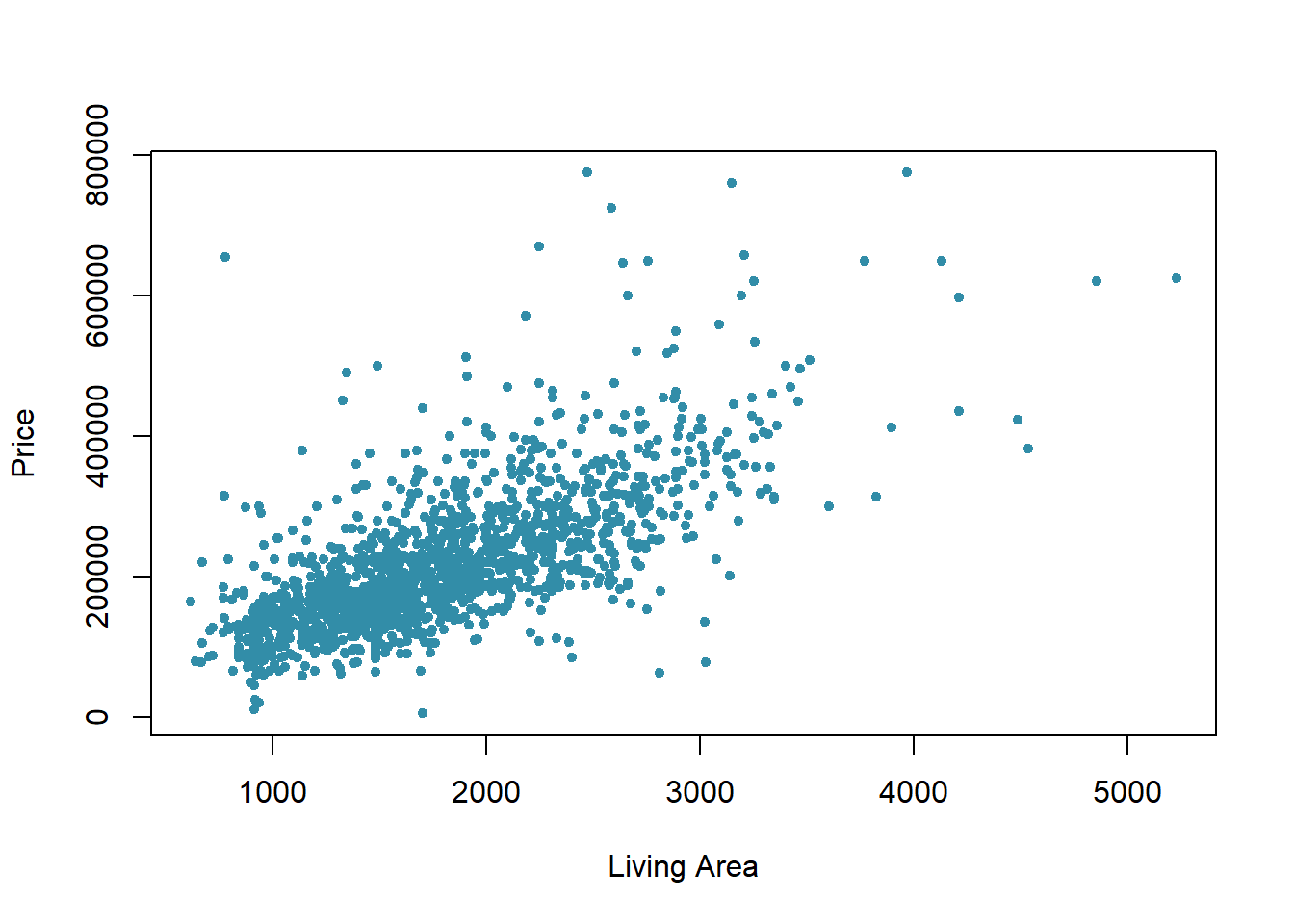

#CC14 part b

options(scipen=1, digits=2)
mod0=lm(Price~Living.Area,data=real)
mod0


Call:
lm(formula = Price ~ Living.Area, data = real)

Coefficients:
(Intercept)  Living.Area  
      13439          113

OK, that new code chunk works to give us a scatter plot and the equation of the line.

But let's run it again using a more familiar code chunk from the Correlation Rehearse:

#CC15 part a

cor(real$`Living.Area`,
    real$`Price`)

[1] 0.71

#CC15 part b

ggplot(real, aes(x=`Living.Area`,
                     y=`Price`))+
  geom_point(col="#328da8")+
  geom_smooth(method=lm, se=FALSE)+
  theme_classic()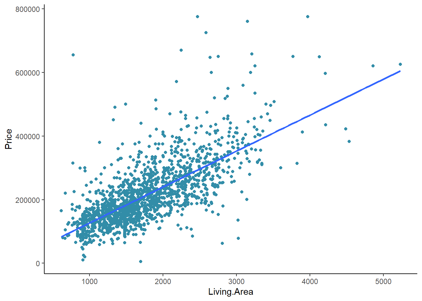

Reflection

How weak or strong do you consider the correlation between Price and Living Area? See Table 1 in this NIH reference

Your answer here:

4.5 Equation of the regression line

Using the two values from CC14 part b, we can develop the equation of the trend line: y = 113*x + 13439, where y is the price of the house and x is the living area of the home. Thus, a home with 1000 SF would be priced at $113 times 1,000 + $13,439. Or 113,000 + 13,439 which is approximately $126,000.

Let's plot the best fit straight line and try to distinguish the houses with and without fireplaces.

If we model the relationship between Price on Living Area with a linear regression, the model shows a slope of 113 which means that each additional square foot is associated with a Price increase of about $113:

Are the houses with fireplaces evenly distributed in this scatter plot? Let's color the ones with fireplaces orange:

Are the houses with fireplaces evenly distributed in this scatter plot? Let’s color the ones with fireplaces orange:

CC16

colors=rep("pink",length(real$Fireplace))
colors[real$Fireplace=="No"]="#328da8"
colors[real$Fireplace=="Yes"]="#FFA500"
with(real,plot(Price~Living.Area,pch=20,col=colors,xlab="Living Area",ylab="Price"))
abline(mod0)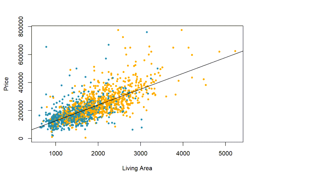

Yes, we have swapped out the old y = mx + b for fancy Greek letters statisticians prefer, but the basic format is still there.

b, the intercept, is now . This is the Greek letter Betta, so this is Betta 0.

m, the coefficient for x is now the Greek letter Beta 1.

And we have added a new term,

Epsilon is the Greek letter for e which represents the error in our equation.

Recall that we are trying to make a best fit line which predicts a value of y for each value of x. Invariably, there will be some error. Don’t worry about this too much. If you take a more advanced course someday, they will likely get into more details about the error or residuals as they are often called.

Again - don’t get too deep in the weeds in this explanation. Just try to read it and get a “feel” for what we are doing. If in the future you take a more advanced course, you will get into this in more depth.

Enough of the background. Let’s run some code.

CC17

mod1=lm(Price~Living.Area+(Fireplace=="Yes"),data=real)
options(scipen=1,digits=2)
summary(mod1)


Call:
lm(formula = Price ~ Living.Area + (Fireplace == "Yes"), data = real)

Residuals:
    Min      1Q  Median      3Q     Max 
-271421  -39935   -7887   28215  554651 

Coefficients:
                       Estimate Std. Error t value Pr(>|t|)    
(Intercept)            13599.16    4991.70    2.72   0.0065 ** 
Living.Area              111.22       2.97   37.48   <2e-16 ***
Fireplace == "Yes"TRUE  5567.38    3716.95    1.50   0.1344    
---
Signif. codes:  0 '***' 0.001 '**' 0.01 '*' 0.05 '.' 0.1 ' ' 1

Residual standard error: 69100 on 1725 degrees of freedom
Multiple R-squared:  0.508, Adjusted R-squared:  0.508 
F-statistic:  891 on 2 and 1725 DF,  p-value: <2e-16

CC18

colors=rep("pink",length(real$Fireplace))
colors[real$Fireplace=="No"]="#328da8"
colors[real$Fireplace=="Yes"]="#FFA500"
with(real,plot(Price~Living.Area,pch=20,col=colors,xlab="Living Area",ylab="Price"))
abline(mod1,col="#328da8")
abline(c(19167+5567,111),col="#FFA500")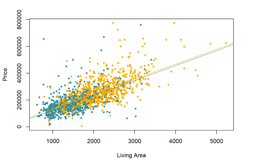

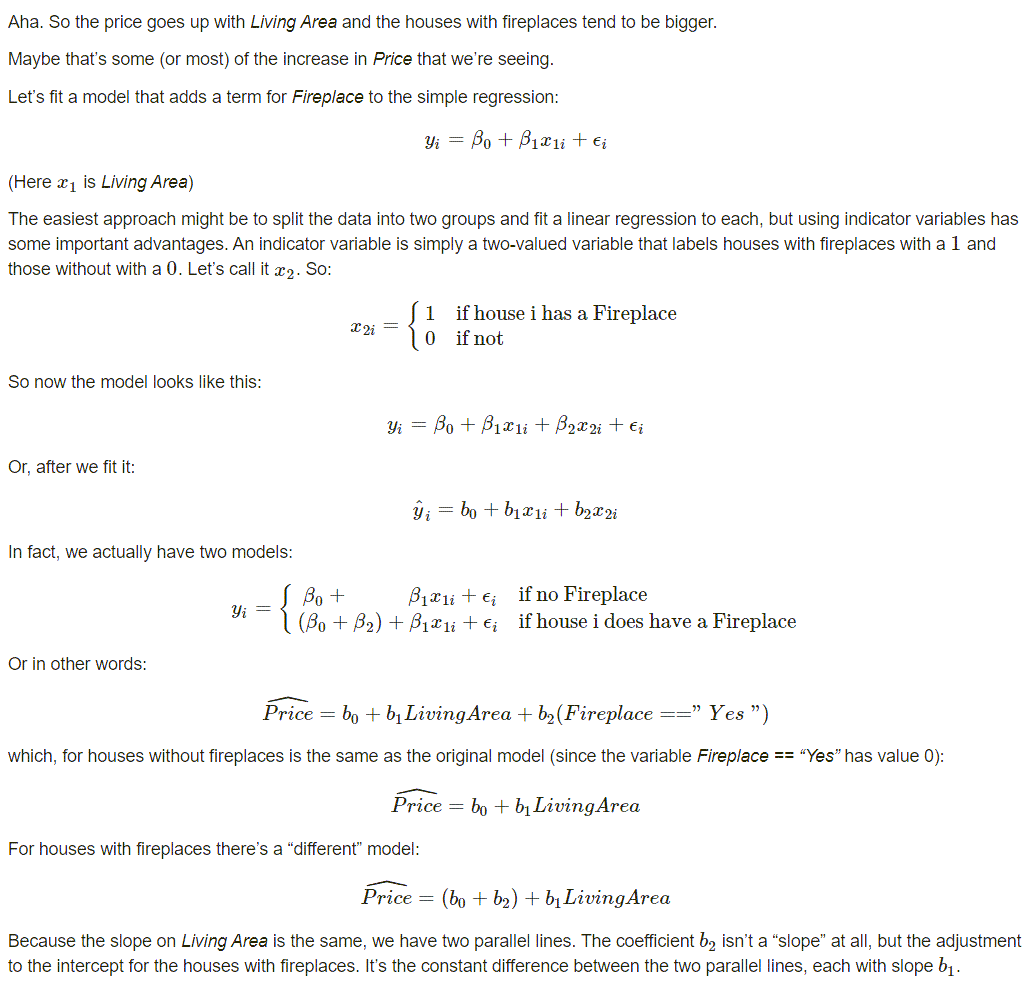
So, it seems a fireplace might adds about $5567, on average to the Price, not $65,000, if we adjust for the size of the house. We can see this as the difference between the two slopes of the regression lines, one for houses with fireplaces, and one for those without. They are parallel and just a bit apart on this chart.

Do we need the intercept adjuster?

We can test to see if we need β2 just like any coefficient by looking at its p-value. We will dig into this concept in a later module, but for now just understand we can check to see if the intercept adjuster is statistically significant. If it is not, we can safely ignore it.

And it turns out this intercept adjuster we can ignore. But something else is going on we need to investigate next.

4.6 Are the slopes the same?

Of course, in this model, we’ve assumed that the difference in price between houses with and without fireplaces is constant, no matter what their size. Let’s let this assumption go by adding an interaction term and adding it to the model.

We do that by multiplying the indicator variable by the quantitative term:

Or we can state the equation as

Price = b0 + b1 times x1 + b2 times x2 + b3 times x3

Again, for the houses without fireplaces, both the x2 and x3 terms will be zero, so, for them, we’ll still have:

Price = b0 + b1 times Living Area

But for houses with fireplaces Fireplace ==“Yes” is 1, and so:

Price = (b0 + b2) + (b1 + b3) times Living Area

The term b2 acts as an intercept adjuster for houses with fireplaces, and the new interaction term b3 acts as a slope adjuster:

CC19

mod2=lm(Price~Living.Area+Fireplace+Living.Area*Fireplace,data=real)
options(scipen=1,digits=2)
summary(mod2)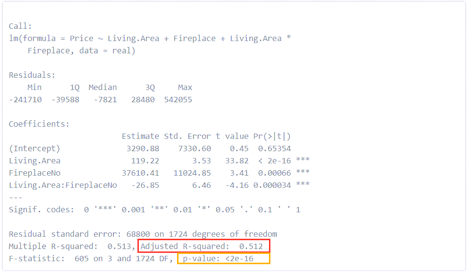

Don’t get lost in the weeds of this output, just trust that the results are statistically significant and we can use this model to give us better estimates of the price of homes with and without fireplaces if we just use the Living Area. In a coming module we will look more deeply at just what “statistically significant means and how we test for it.

For right now, we do want to call out two important values in this linear regression output.

In the smaller orange box, we have the p-value which tells us whether or not the regression is statistically significant. Small values indicate significance. Here, in scientific notation again, is a p-value that is very, very small.

In the larger red box, we have R-squared. This is the Goodness of Fit which tells us how much of the variation in the dependent variable, home price, is accounted for by the regression equation with our two independent variables, Fireplace and Living Area. We have an R-squared of 0.51 which tells us the regression accounts for about 51% of the variation in price. And that tells us something besides living area and fireplace is responsible for the other 49% in price!

This is an important lesson. It’s often true that a more complex model will reveal insights and patterns that a simpler model fails to show.

But let’s look one more time at our regression model. By adding a term allowing the slopes of regression lines of houses with and without fireplaces to vary.

What does this model look like?

CC20

colors=rep("pink",length(real$Fireplace))
colors[real$Fireplace=="No"]="#328da8"
colors[real$Fireplace=="Yes"]="#FFA500"
with(real,plot(Price~Living.Area,pch=20,col=colors,xlab="Living Area",ylab="Price"))
coefs=coefficients(mod2)
abline(c(coefs[1],coefs[2]),col="#FFA500")
abline(c(coefs[1]+coefs[3],coefs[2]+coefs[4]),col="#328da8")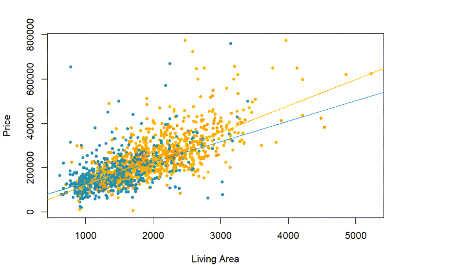

4.7 So, how much is a fireplace worth?

Well, we still can’t assign causality, but it certainly seems that the answer is at least “it depends”. Fireplaces are associated with generally higher prices for large houses, and the bigger the house, the more a fireplace seems to increase the price, but for smaller houses, it seems that the prices are not increased as much with a fireplace.

The lines actually appear to cross at about 1500 SF.

Reflection

Would it be reasonable to conclude that adding a fireplace to a very small house would actually decrease its price? Why or Why not?

Hint: Could it be that there is some uncertainty in the slopes of the two lines? We will discuss confidence intervals around our estimates in the next module.

Your answer here:

5 What have we Learned?

We’ve seen that basing our analysis on simple models and simple averages can lead to incorrect conclusions.

Even though complex models can never prove causality, they can offer explanations that are more plausible that relying on looking at one variable at a time.

We’ve built the model through a series of steps:

Examining the Distribution of a Variable
Comparing two groups via boxplots and summary statistics
Summarizing the relationship between variables using a multiple linear regression
Using indicator variables to adjust models
Using interaction terms (multiplying an indicator variable by a quantitative variable) to create a more complex and realistic model.

Lab Assignment Submission

Important

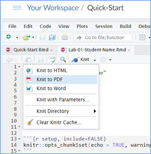
When you are ready to create your final lab report, save the Lab-04-Rehearse-2-Worksheet.Rmd lab file and then Knit it to PDF or Word to make a reproducible file. This image shows you how to select the knit document file type.

Note that if you have difficulty getting the documents to Knit to either Word or PDF, and you cannot fix it, just save the completed worksheet and submit your .Rmd file.

Ask your instructor to help you sort out the issues if you have time.

Submit your file in the M4.3 Lab 4 Rehearse(s): Exploring Relationships assignment area.

The Lab 4 Exploring Relationships Grading Rubric will be used.