Downey/Infer Chi-square Goodness of Fit Test

This is based upon the example here https://infer.netlify.app/articles/observed_stat_examples.html#one-categorical-2-level---gof

The Goodness of Fit Test is used when there is one categorical variable of interest that has more than two levels.

Packages

Load the packages into the library!

cc4

library(tidyverse)
library(infer)

Note: there are three code chunks which are hidden. Thus this is cc4.

To make this example reproducible we use the set.seed() function.

cc5

#make this example reproducible
set.seed(1)

Initial Steps

For every research question analysis, there are things to do when you begin.

State your research question/problem statement

A particular brand of candy-coated chocolate comes in five different colors: brown, coffee, green, orange, and yellow.

The manufacturer of the candy claims the candies are distributed in the following color proportions:

brown - 40%
coffee - 10%.
green - 10%
orange - 20%
yellow - 20%

Hint: It is best practice to arrange the names of the levels of categorical variables in alphabetical order because some functions assume that to be true - data is arranged in alphabetical order.

A random sample of 600 pieces of this candy is collected.

The specific research question is: Does this random sample of the candies provide sufficient evidence against the manufacturer’s claim such that it should be rejected?

State the Null and Alternative hypotheses

Null hypothesis: The true proportions of a particular brand of candy-coated chocolate match what the manufacturer states: brown - 40%, coffee - 10%, green - 10%, orange - 20%, yellow - 20%.

Alternative hypothesis: The distribution of candy proportions differs from what the manufacturer states.

State the Significance Level

It’s important to set the significance level “alpha” before starting the testing using the data.

Let’s set the significance level at 5% ( i.e., 0.05) here because nothing too serious will happen if we are wrong. (we are not going to publish our results!)

Get Familiar with the data

Load the data

Read in and inspect the data. The data file (candies02.csv) is located in the /data folder. The following code chunk reads in the original csv file from the /data folder and creates a new data object named candies.

cc6

candies <- read.csv("./data/candies02.csv")

Inspect the data

Look at the top of the data object candies.

cc7

head(candies)

##   color_
## 1  brown
## 2  brown
## 3  brown
## 4  brown
## 5  brown
## 6  brown

The data object candies contains one column/variable named color_.

The values in the rows are names of candy colors. Thus color_ is categorical variable with five levels (the five color names).

Let’s look at the end of the data:

cc8

tail(candies)

##     color_
## 595 yellow
## 596 yellow
## 597 yellow
## 598 yellow
## 599 yellow
## 600 yellow

But we cannot see all the colors, so click on the candies data object in the Environment to open it in the Source window and scroll down to see all five colors.

Find the counts

Find the counts of each color observed:

cc9

color_count <- table(candies$color_)
color_count

## 
##  brown coffee  green orange yellow 
##    234     60     48    132    126

Find observed proportions

cc10

obs_prop <- prop.table(table(candies$color_))
obs_prop

## 
##  brown coffee  green orange yellow 
##   0.39   0.10   0.08   0.22   0.21

Visualize the data

In the following code chunk, we create a bar chart to display the count of the number of M&M’s of each of the stated colors in the dataset candies.

cc11

ggplot(data = candies, aes(x = color_, fill = color_)) +   geom_bar()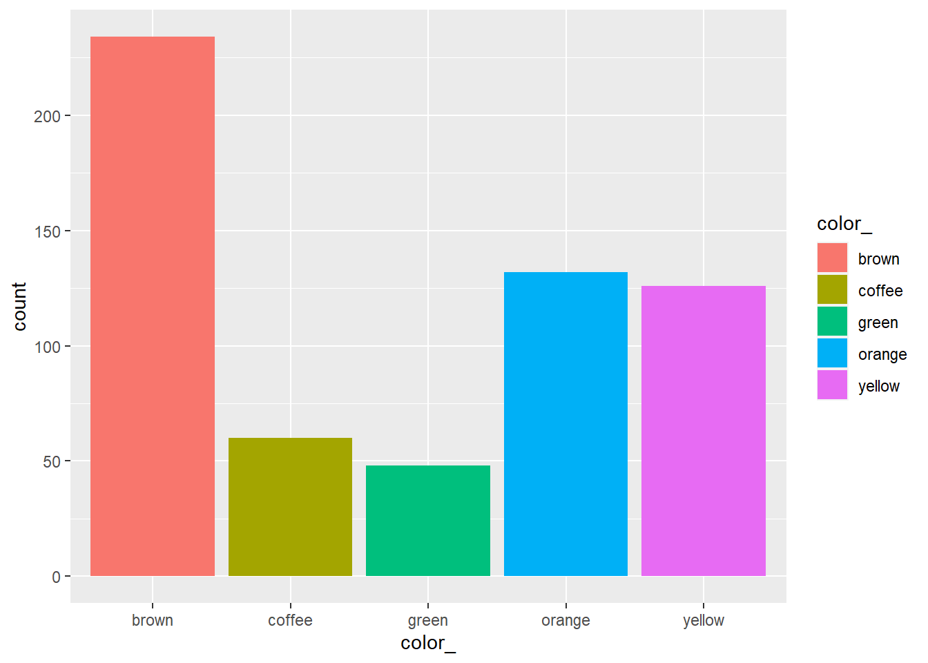

Note that in the last code chunk we allowed R to select the color. That is why most of the colors do not match the actual color names.

We can use standard codes for the colors, called “hex codes.” There are several places where you can get the hex codes. Here is one site that has several easy to use ways to pick color code: https://htmlcolorcodes.com/ We used this page to pick the brown and coffee color hex codes https://htmlcolorcodes.com/colors/shades-of-brown/

cc11 improved version

ggplot(data = candies, aes(x = color_, fill = color_)) +   geom_bar() +
  scale_fill_manual(values=c("#8B4513", "#6F4E37", "#50C878", "#FFAC1C", "#FFEA00"))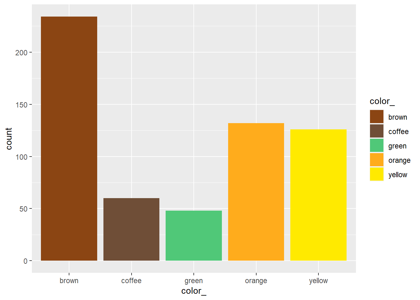

Stacked Bar Chart

Important

You do not need to include this chart - it is for information purposes only.

We wrangled the data to create a special data set to create a stacked bar chart to better illustrate the Planned and Observed proportions of colors of candies. We will use it for this chart only.

cc12

candies2 <- read.csv("./data/candies2.csv")

cc13

candies2 %>% ggplot(aes(x = group, fill = color_)) +
  geom_bar(position = "fill") +
  #the values are the "Hex" codes for brown, coffee, green, orange, and yellow.
  scale_fill_manual(values=c("#8B4513", "#6F4E37", "#50C878", "#FFAC1C", "#FFEA00")) +
  ylab("Proportion") +
  xlab("Observed vs Planned Proportions") +
  ggtitle("Proportions of Colors")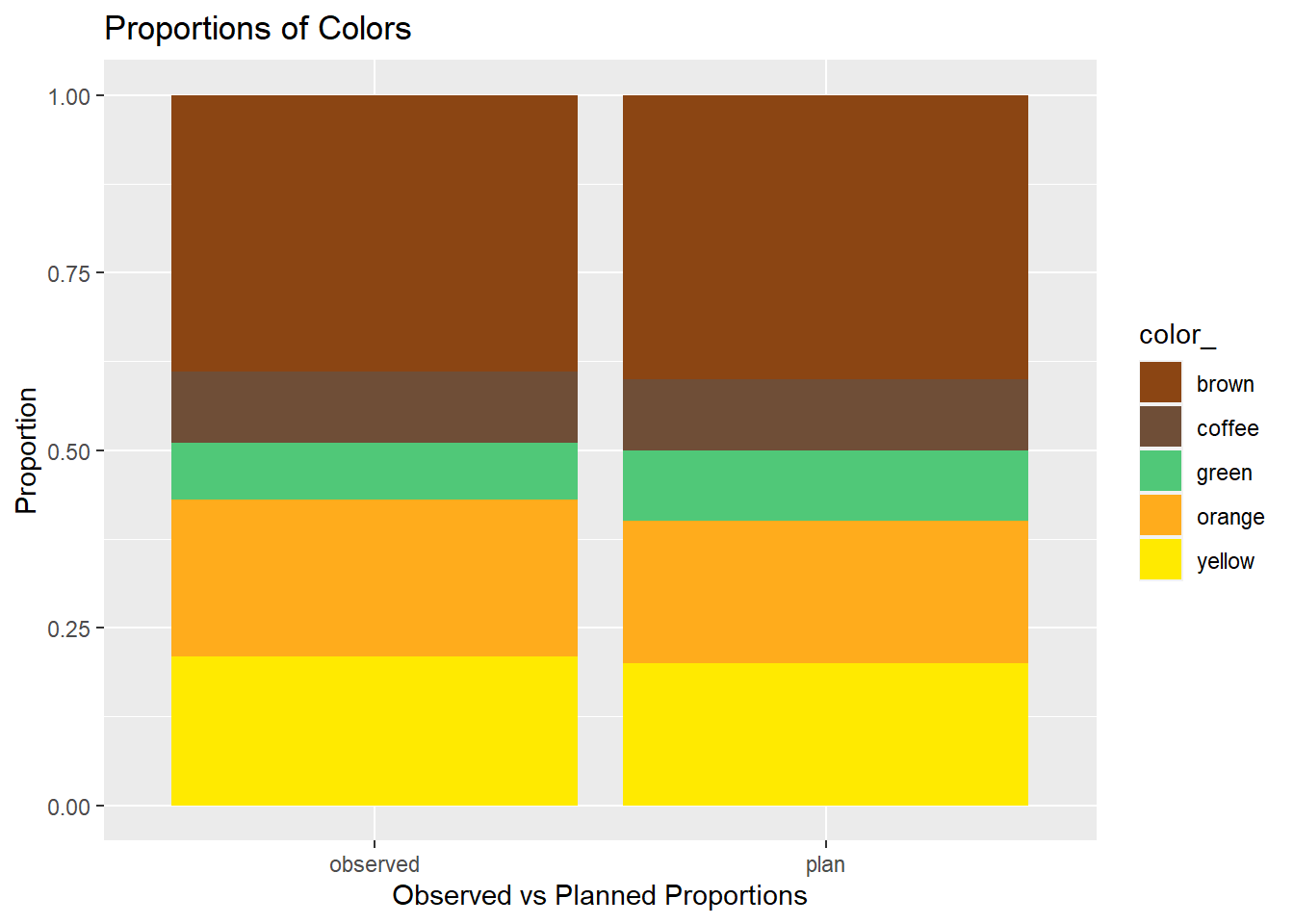

What does the stacked bar chart indicate to you?

Your Answer here:

The Downey/Infer Steps

Downey’s 5 INFER steps:

Specify: Calculate a sample statistic, or “delta.”
Generate: Use simulation to invent a world where “delta” is null.
Visualize: Look at “delta” in the null world.
Calculate the probability that “delta” could exist in null world.
Decide if “delta” is statistically significant.

1 Specify and Calculate

Find the observed test statistic “delta.”

We use the Chi-square statistic for our difference Delta.

Note that we use a “point” null even though we have five values - they are all point values.

It is important that the sum of the proportions values add up to exactly 1.

cc14

Delta <- candies %>%
#specify response variable
   specify(response = color_) %>%
#use the Null values here, not the observed proportions 
  hypothesize(null = "point",
              p = c("brown" = 0.4,
                    "coffee" = 0.1,
                    "green" = 0.1,
                    "orange" = 0.2,
                    "yellow" = 0.2)) %>%
  calculate(stat = "Chisq")

Delta

## Response: color_ (factor)
## Null Hypothesis: point
## # A tibble: 1 × 1
##    stat
##   <dbl>
## 1  4.05

Our observed difference Delta equals a Chi-square value of 4.05.

2 Generate

Generate the Null distribution

cc15

null_dist <- candies %>%
#specify response variable
   specify(response = color_) %>%
#use the Null proportions here
  hypothesize(null = "point",
              p = c("brown" = 0.4,
                    "coffee" = 0.1,
                    "green" = 0.1,
                    "orange" = 0.2,
                    "yellow" = 0.2)) %>%
  #the next line is added to generate the 1000 reps for the Null Distribution
  generate(reps = 1000, type = "draw") %>%
  calculate(stat = "Chisq")

3 Visualize

Visualize the observed statistic Delta and the Null distribution

cc16

visualize(null_dist) +
#Note the Chi-square test is always a right-tail test
  shade_p_value(obs_stat = Delta, direction = "greater")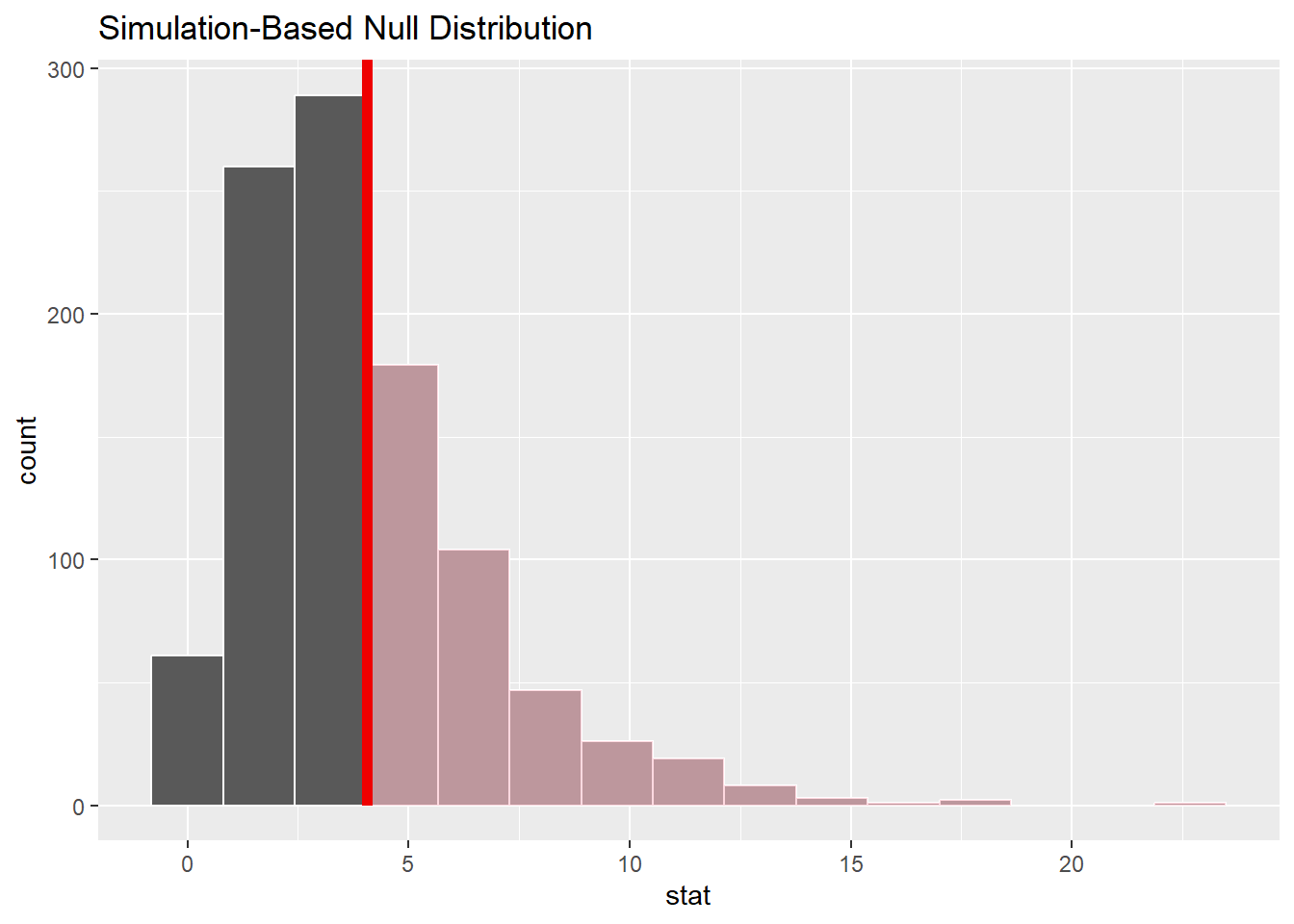

The observed test statistic of 4.05 does not appear to be in the “tail” of the null distribution and thus is not unusual.

Remember that the “pinkish” shaded portion of the distribution represents the area under the “curve” and thus the probability of getting an as extreme (extreme means ‘large value’ since the Chi-square test is always a right-tail test) or even more extreme delta - i.e. the p-value.

4 p-value

Calculate the p-value (“area” under the curve beyond Delta) from the Null distribution and the observed statistic Delta.

cc17

null_dist %>%
  get_p_value(obs_stat = Delta, direction = "greater")

## # A tibble: 1 × 1
##   p_value
##     <dbl>
## 1    0.39

5 State Conclusion

Because the p-value of 0.39 is not less than the significance level of 0.05, we cannot reject the Null Hypothesis that the observed distribution of proportions of candy colors is the same as the planned distribution of proportions of candy colors.

Traditional Method

Check using the traditional Chi-square test included in the Infer package.

cc18

chisq_test(candies,
  response = color_,
  p = c("brown" = 0.4,
        "coffee" = 0.1,
        "green" = 0.1,
        "orange" = 0.2,
        "yellow" = 0.2))

## # A tibble: 1 × 3
##   statistic chisq_df p_value
##       <dbl>    <dbl>   <dbl>
## 1      4.05        4   0.399

The Infer and Traditional methods produce similar results, but of course we would need to check all the assumptions for the traditional method.

No need for that with Downey/Infer!

Follow this link back to the Chi-square Test for Independence

Lab 7 Rehearse 2

Chi-square Tests for Multiple Proportions