Lab 3 Remix & Report

Click this Link:

Log into your Posit Cloud account.
Open the Lab 3 Distributions project.
Open the Lab-03-Student-Name.Rmd.

In this lab, we are going to combine the Remix and Report. This is similar to what happens in many research papers and reports to management.

All the instructions below are also in your Lab-03-Student-Name.Rmd file. So, you can open that file in your Posit Cloud, and just follow the instructions in the template and close/minimize this browser window if you want.

**IMPORTANT!

Remember to rename this file to include your name in place of “Student-Name” at the top of the page. Also, change the date to the current date inside the file.

Other than entering your name to replace Student Name and changing the date to the current date, do not change anything in the head space.

Load the libraries!

The code is in the report template, so just run it.

library(ggplot2)
library(tidyverse)
library(moderndive)
library(scales)

We are going to set the random number generator seed to a different value than in Rehearse 2. This may mean you get different values when you run code chunks later in this Remix.

# Set output digit precision
options(scipen = 99, digits = 3)

# Set random number generator see value for replicable pseudorandomness

set.seed(75)

Remix

In section 3.2.2 Virtual Sampling of Lab 3 Rehearse 2, we took virtual samples with three different sample sizes: 25, 50, and 100.

For this Remix, select a sample size between 10 and 90, not using the 25 or 50 sample sizes, and then rerun the code using your new sample size.

You need to edit the code chunk below, carefully replacing every instance of XX in the chunk with your chosen sample size.

# Segment 1: sample size = XX 

# 1.a) Virtually use shovel 1000 times
virtual_samples_XX <- bowl %>% 
  rep_sample_n(size = XX, reps = 1000)

# 1.b) Compute resulting 1000 replicates of proportion red
virtual_prop_red_XX <- virtual_samples_XX %>% 
  group_by(replicate) %>% 
  summarize(red = sum(color == "red")) %>% 
  mutate(prop_red = red / XX)

# 1.c) Plot distribution via a histogram
ggplot(virtual_prop_red_XX, aes(x = prop_red)) +
  geom_histogram(binwidth = 0.05, boundary = 0.4, color = "white") +
  labs(x = "Proportion of XX balls that were red", title = "25")

Run the code several times paying attention to the shape and approximate center of the histogram each time.

Q1.

What is the approximate mean of the histogram for your sample size of XX?

Your answer here:

Q2.

How does the variation - shape - of the histogram differ from the shape of the original n = 100 sample size?

Here is CC10 from Lab 3 Rehearse 2 which plots the histogram for a sample size of n = 100:

# Segment 3: sample size = 100 ------------------------------
# 3.a) Virtually using shovel with 100 slots 1000 times
virtual_samples_100 <- bowl %>% 
  rep_sample_n(size = 100, reps = 1000)

# 3.b) Compute resulting 1000 replicates of proportion red
virtual_prop_red_100 <- virtual_samples_100 %>% 
  group_by(replicate) %>% 
  summarize(red = sum(color == "red")) %>% 
  mutate(prop_red = red / 100)

# 3.c) Plot distribution via a histogram
ggplot(virtual_prop_red_100, aes(x = prop_red)) +
  geom_histogram(binwidth = 0.05, boundary = 0.4, color = "white") +
  labs(x = "Proportion of 100 balls that were red", title = "100")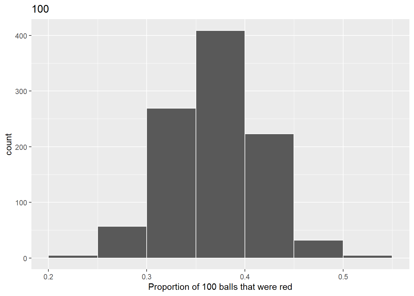

To calculate the standard deviation for sample size n = 100, rerun this code chunk 13 from Lab 3 Rehearse 2 section 3.2.2.

# n = 100
virtual_prop_red_100 %>% 
  #summarize(sd = sd(prop_red)) %>%
  summarise(mean = mean(prop_red),
            sd = sd(prop_red))

# A tibble: 1 × 2
   mean     sd
  <dbl>  <dbl>
1 0.375 0.0460

Be sure to change every instance of “XX” comment in the code chunk below to calculate the standard deviation for your new sample size n.

# n = XX
virtual_prop_red_XX %>% 
  summarise(mean = mean(prop_red),
            sd = sd(prop_red))

Write your Q2 answer here:

Z-scores

In section 3.9 of the Distribution Rehearse, we discussed z-scores. Let’s expand on this idea a bit.

One common task is to describe an observation in relation to the distribution of all the observations. You can do this by finding the z-score. If you convert individual observations to z-scores, you can compare observations from different distributions.

Times for 5k and 10k runs are approximately normally distributed. That tells us the histogram of times is bell shaped and roughly symmetrical.

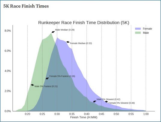
Image by Chris Drouin in Medium using Runkeeper data 2017 (Drouin, 2017)

Q3.

Lian ran a 10k run this week in 45 minutes. The mean time for women runners her age in this race was 50 minutes and the standard deviation was 5 minutes. Using the z-score formula, what is Lian’s z-score on the 10k race?

Edit the blue numbers in this code appropriately

Lian1<-11
racemean1 <-22
racesd1 <-33
Liandifference1 <-Lian1-racemean1
Lianz1<-Liandifference1/racesd1
print(Lianz1)

0
-1
+1
-2

Your answer here:

Q4.

Last week, Lian finished a 5k run in 39 minutes. The mean time for women her age for that run is 33 minutes, and the standard deviation is 3 minutes. Using the z-score formula, what is Lian’s z-score on the 5k race?

0
-1
+1
+2

Remember to edit the blue numbers again.

Lian2<-11
racemean2 <-22
racesd2 <-33
Liandifference2 <-Lian2-racemean2
Lian2z<-Liandifference2/racesd2
print(Lian2z)

Your answer here:

Q5.

On which race did Lian do the better compared to the mean time of women?

5k race
10k race
Lian did equally well on both races.

Explain your choice.

Your answer here:

Report

You answered a lot of reflection questions in the two rehearses. So, just two questions here:

Q6.

Explain the concept of sampling error.

your answer here:

Q7.

Explain why the standard deviation of the sampling distribution of mean gets smaller as sample-size increases,

your answer here:

** Just about done!**

As you did Labs 01 and 02, when you have edited the code chunks, you need to Knit it so see the updated graphs and tables in your final report. When you Knit an Rmarkdown file, any code chunks in it are automatically run. And all data objects in the Environment are ignored.

Lab Assignment Submission

Important

When you are ready to create your final lab report, save the Lab-3-Remix-Your-Name.Rmd lab file and then Knit it to PDF or Word to make a reproducible file. This image shows you how to select the knit document file type.

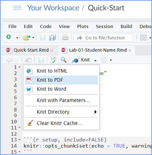
If you cannot knit to either a Word or PDF file, and you cannot fix it, just save the completed worksheet and submit your Lab-03-Remix-Your-Name.Rmd file for partial credit.

Ask your instructor to help you sort out the issues if you have time.

Submit your file in the M3.4 Lab 3 Remix and Report: Sampling, Distributions and Central Limit Theorem assignment area.

The Lab 3 Grading Rubric will be used.